MATH 565 — Fall 2026
Selected Topics
October 9, 2026
Course Map

Probability
Statistics
Analysis
Computer
Science
Science
Estimation
Error
Assessment
Assessment
Variance
Reduction
Reduction
Multilevel
Monte Carlo
Monte Carlo
Stochastic
Optimization
Optimization
High-Performance
Computing
Computing
Course decks
Share the work across processors, samples, and levels
Parallel and Stochastic Computation
Practice
Parallel computing
Practice
Modern CPUs and GPUs can evaluate many operations concurrently
- Monte Carlo function values are often pleasingly parallel: samples can be evaluated independently
- Parallel random-number streams must remain nonoverlapping and statistically sound
- GPU arithmetic is often optimized for 32-bit floating point rather than 64-bit floating point
- Reduced precision may lose significant digits but can increase throughput substantially
- GPUs help most when there are many similar operations
Launch and data-transfer costs can dominate small problems
Parallelism changes computational cost
It does not repair biased estimators or poor sampling designs
Gradient descent
Estimation
For
\[ \vtheta_* = \argmin_{\vtheta\in\reals^m}\operatorname{Loss}(\vtheta), \]
gradient descent iterates
\[ \vtheta_{k+1}=\vtheta_k-\eta_k\nabla\operatorname{Loss}(\vtheta_k) \]
- \(\eta_k\) is the step size or learning rate
- The loss often decreases toward a local minimum
- Curvature-aware methods can use second derivatives
Each step becomes more expensive - Step sizes that are too large may overshoot
Step sizes that are too small converge slowly
Move downhill using all available data
Stochastic gradient descent
Estimation
Suppose
\[ \operatorname{Loss}(\vtheta) =\sum_{i=0}^{N-1}\operatorname{loss}_i(\vtheta) \]
Computing the full gradient costs \(N\) component gradients
Stochastic gradient descent uses an inexpensive random component:
\[ \vtheta_{k+1}=\vtheta_k-\eta_k\nabla\operatorname{loss}_{I_k}(\vtheta_k), \qquad I_k\sim\Unif\{1,\ldots,N\} \]
Common variants include
- decaying learning rates
- mini-batch gradients
- mini-batches with decay
The stochastic gradient is cheap but noisy
Averaging a mini-batch reduces its variance
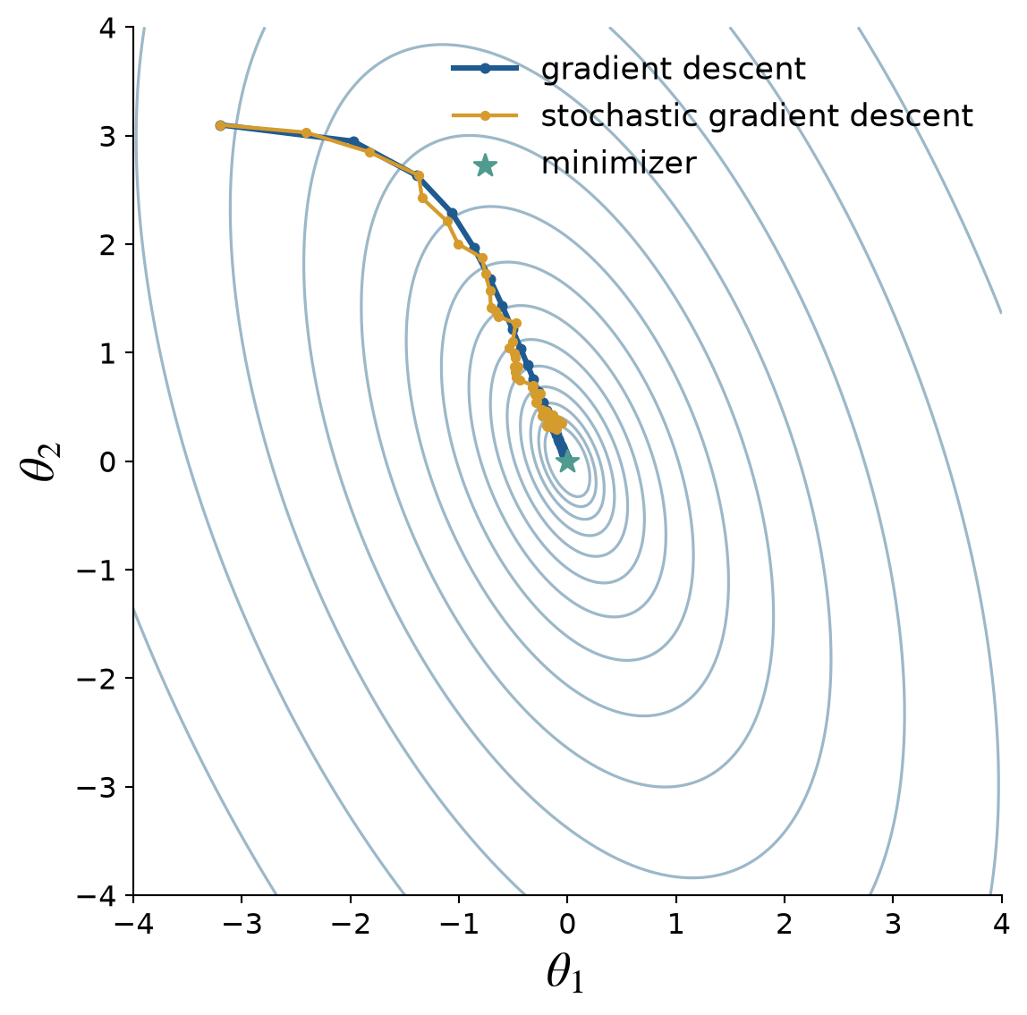
Gradient and stochastic-gradient paths
Estimation
Both methods minimize the same quadratic loss
Stochastic gradients use one randomly selected component at each step
Two-Level Monte Carlo
Estimation
Splitting an expectation
Estimation
Suppose
\[ Y=Y_1+Y_2, \qquad \mu=\mu_1+\mu_2, \qquad \mu_\ell=\Ex(Y_\ell) \]
Estimate the two means independently:
\[\begin{align*} \hmu&=\hmu_1+\hmu_2,& \hmu_\ell&=\frac1{n_\ell}\sum_{i=0}^{n_\ell-1}Y_{i\ell} \end{align*}\]
If one sample of \(Y_\ell\) costs \(\$_\ell\), then
\[\begin{align*} \mse(\hmu) &=\frac{\var(Y_1)}{n_1}+\frac{\var(Y_2)}{n_2},\\ \cost(\hmu)&=n_1\$_1+n_2\$_2 \end{align*}\]
The sample counts should reflect both variance and cost per sample
Allocating work optimally
Estimation
For a fixed total cost \(C\), minimize
\[ \frac{V_1}{n_1}+\frac{V_2}{n_2} \quad\text{subject to}\quad n_1\$_1+n_2\$_2=C, \qquad V_\ell=\var(Y_\ell) \]
The optimal ratio is
\[ \frac{n_1}{n_2} =\sqrt{\frac{V_1\$_2}{V_2\$_1}} \]
and the optimal mean squared error is
\[ \mse(\hmu) =\frac1C\left(\sqrt{V_1\$_1}+\sqrt{V_2\$_2}\right)^2 \]
Use more samples at a level with larger variance and fewer samples at a level with larger cost
What two levels accomplish
Estimation
- Larger \(\var(Y_\ell)\) implies a larger optimal \(n_\ell\)
- Larger cost \(\$_\ell\) implies a smaller optimal \(n_\ell\)
- Pilot samples can estimate unknown variances and costs
- Often \(\mu=\mu_1+\mu_2\), where
- \(Y_1\) is a cheap approximation sampled often
- \(Y_2\) is an expensive correction sampled less often
The decomposition is useful when the expensive correction has small variance
Multilevel Monte Carlo
Estimation
Many levels
Estimation
Let
\[ Y=Y_1+\cdots+Y_L, \qquad \mu=\sum_{\ell=1}^L\mu_\ell, \qquad \mu_\ell=\Ex(Y_\ell) \]
With independent samples at each level,
\[\begin{align*} \hmu&=\sum_{\ell=1}^L\hmu_\ell,& \hmu_\ell&=\frac1{n_\ell}\sum_{i=0}^{n_\ell-1}Y_{i\ell},\\ \mse(\hmu)&=\sum_{\ell=1}^L\frac{V_\ell}{n_\ell},& \cost(\hmu)&=\sum_{\ell=1}^Ln_\ell\$_\ell \end{align*}\]
The challenge is to choose both the level decomposition and the sample allocation
Optimal multilevel allocation
Estimation
For total cost \(C\), the optimal allocation is proportional to
\[ n_\ell\propto\sqrt{\frac{V_\ell}{\$_\ell}} \]
More explicitly,
\[ n_\ell =\frac{C\sqrt{V_\ell/\$_\ell}} {\sum_{k=1}^L\sqrt{V_k\$_k}} \]
The resulting mean squared error is
\[ \mse(\hmu) =\frac1C\left(\sum_{\ell=1}^L\sqrt{V_\ell\$_\ell}\right)^2 \]
Efficiency depends on keeping \(V_\ell\$_\ell\) small across levels
Infinite-dimensional expectations
Estimation
Suppose
\[ \mu=\lim_{d\to\infty}\Ex\{f_d(\vX_{1:d})\} \]
as in an option payoff based on an increasingly fine time discretization
Choose \(d_1<\cdots<d_L\) and define coupled differences
\[\begin{align*} Y_1&=f_{d_1}(\vX_{1:d_1}),\\ Y_\ell&=f_{d_\ell}(\vX_{1:d_\ell}) -f_{d_{\ell-1}}(\vX_{1:d_{\ell-1}}), \qquad \ell\ge2 \end{align*}\]
Then
\[ \Ex\{f_{d_L}(\vX_{1:d_L})\} =\sum_{\ell=1}^L\Ex(Y_\ell) \]
with a remaining truncation bias \(\mu-\Ex\{f_{d_L}(\vX_{1:d_L})\}\)
Why telescoping helps
Estimation
- Fine approximations are expensive
- Coupling makes adjacent approximations similar
- Their difference \(Y_\ell\) can have rapidly decreasing variance
- Sample cheap, coarse levels many times and expensive, fine corrections fewer times
If \(d_\ell=m^\ell\), \(V_\ell\lesssim\beta^\ell\), and \(\$_\ell\lesssim m^\ell\), then
\[ \sum_{\ell=1}^L\sqrt{V_\ell\$_\ell} \lesssim\sum_{\ell=1}^L(\beta m)^{\ell/2} \]
- If \(\beta m<1\), total stochastic cost is governed mainly by coarse levels
- If \(\beta m>1\), the finest corrections dominate
Multilevel Monte Carlo is effective when correction variance decays faster than correction cost grows
Big Ideas
Probability
Statistics
Estimation
- Monte Carlo samples are naturally parallel, but random streams and precision still matter
- Stochastic gradients trade exact directions for cheaper iterations
- Two-level and multilevel estimators split work according to variance and cost
- Coupling adjacent approximations creates low-variance corrections
- A good hierarchy spends most computation where it buys the largest reduction in error