Metropolis–Hastings Sampling
Markov Chain
The Metropolis–Hastings algorithm
Markov Chain
For states in \(\reals^d\) , suppose
the target has normalized density \(\varrho_{\mathrm{tar}}\) , known up to a factor through \(\widetilde\varrho_{\mathrm{tar}}\propto\varrho_{\mathrm{tar}}\)
\(\varrho_{\mathrm{prop}}(\vz\mid \vx)\) proposes a new state \(\vz\) from the current state \(\vx\)
Given \(\vX_0\) , repeat for \(i=0,\ldots,n-2\) :
Generate \(\vZ_i\mid\vX_i\sim\varrho_{\mathrm{prop}}(\cdot\mid \vX_i)\) and \(V_i\sim\Unif[0,1]\) , independently of the proposal
Compute
\[
\alpha(\vX_i,\vZ_i)=\min\!\left\{1,
\frac{\widetilde\varrho_{\mathrm{tar}}(\vZ_i)\varrho_{\mathrm{prop}}(\vX_i\mid \vZ_i)}
{\widetilde\varrho_{\mathrm{tar}}(\vX_i)\varrho_{\mathrm{prop}}(\vZ_i\mid \vX_i)}\right\}
=\min\!\left\{1,
\frac{\text{joint density of first $\vZ_i$, then $\vX_i$}}
{\text{joint density of first $\vX_i$, then $\vZ_i$}}\right\}
\]
Set \(\vX_{i+1}=\vZ_i\) if \(V_i\le\alpha(\vX_i,\vZ_i)\) \(\vX_{i+1}=\vX_i\)
Every iteration accepts either the proposal or the current state \(Y_i=f(\vX_i)\) for output summaries
Why the acceptance ratio works
Markov Chain
Probability
The ratio compares the two directions of a proposed transition:
\[
\frac{\widetilde\varrho_{\mathrm{tar}}(\vZ_i)\varrho_{\mathrm{prop}}(\vX_i\mid \vZ_i)}
{\widetilde\varrho_{\mathrm{tar}}(\vX_i)\varrho_{\mathrm{prop}}(\vZ_i\mid \vX_i)}
=
\frac{\text{target weight at $\vZ_i$}\times\text{return proposal}}
{\text{target weight at $\vX_i$}\times\text{forward proposal}}
\]
Moves toward higher target density are favored
Asymmetric proposals are corrected by the proposal-density ratio
The unknown factor relating \(\widetilde\varrho_{\mathrm{tar}}\) to the target cancels
Detailed balance preserves the target; convergence from the starting state requires suitable conditions
The Metropolis algorithm
Markov Chain
If the proposal is symmetric,
\[
\varrho_{\mathrm{prop}}(\vz\mid \vx)
=\varrho_{\mathrm{prop}}(\vx\mid \vz),
\]
then the acceptance probability simplifies to
\[
\alpha(\vx,\vz)=\min\!\left\{1,
\frac{\widetilde\varrho_{\mathrm{tar}}(\vz)}{\widetilde\varrho_{\mathrm{tar}}(\vx)}\right\}
\]
For a random-walk proposal \(\vZ_i=\vX_i+\vepsilon_i\) with symmetric \(\vepsilon_i\) :
accept every move to a state with at least as much target density
accept some downhill moves, which keeps the chain from becoming trapped immediately
repeat \(\vX_i\) when a proposal is rejected
Metropolis practice
Practice
Markov Chain
Use the uniform numbers in order and choose a random order of the candidate \(z\) values
\(V_i\) 0.6
0.1
0.3
0.5
0.9
0.2
0.1
0.4
\(\widetilde\varrho_{\mathrm{tar}}(z)\) 0.1
0.8
2.0
1.6
0.5
2.6
2.4
1.0
\(\exstar\) Starting at \(x=-1.2\) , follow several Metropolis steps and record each accepted or repeated state
A random-walk Metropolis example
Practice
Markov Chain
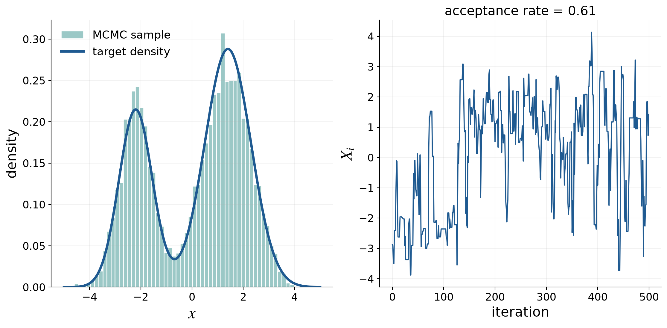
Target a bimodal Gaussian mixture using the symmetric proposal
\[
Z\mid X_i=x\sim\Norm(x,1.4^2)
\]
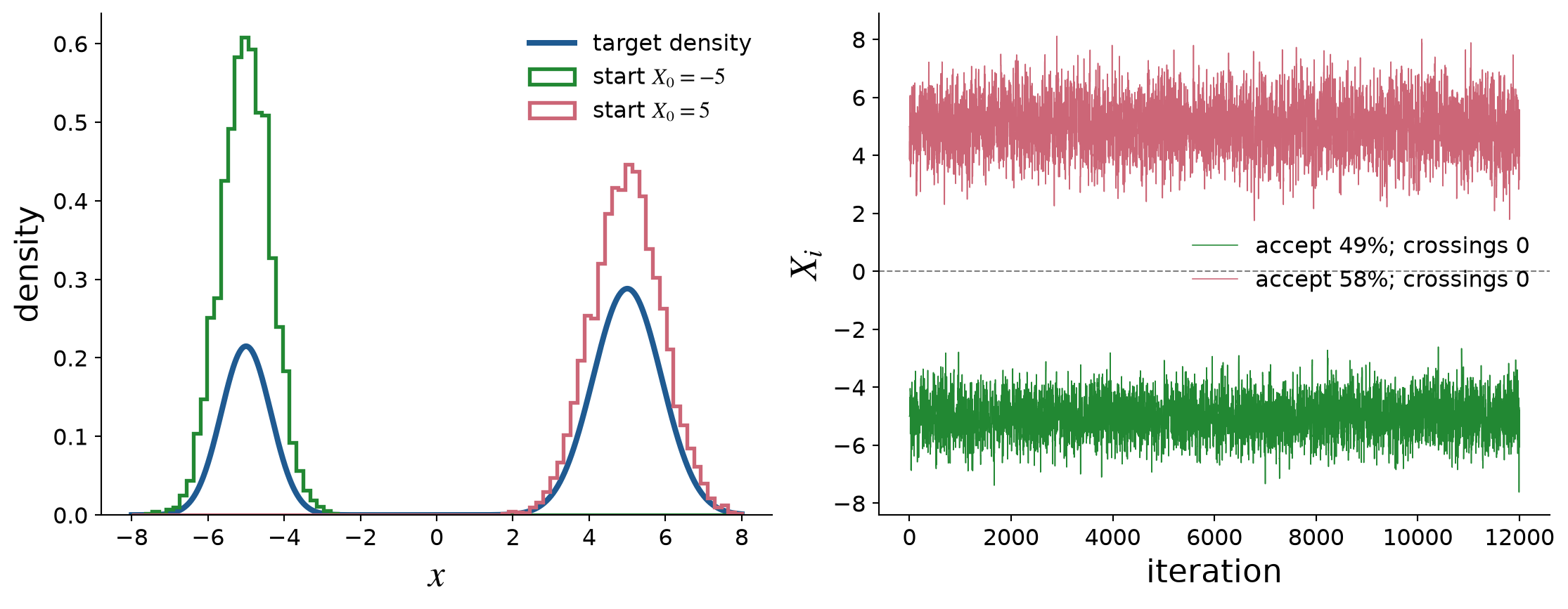
Separated modes can trap a chain
Practice
Markov Chain
Same mixture weights and widths; move the means to \(-5\) and \(5\) \(Z\mid X_i=x\sim\Norm(x,1.4^2)\) ; start one chain in each mode
Acceptance within a mode does not establish exploration of both modes
Tuning and diagnostics
Markov Chain
Statistics
MCMC is attractive because it
samples from complicated, unnormalized target densities
is often straightforward to implement
The proposal and starting point require care:
proposals that are too small explore slowly and produce highly dependent samples
proposals that are too large have low acceptance rates and many repeats
multimodal targets may trap a single chain in one mode
Useful responses include pilot runs , multiple chains , and parallel tempering
MetropolisHastings companion notebook
Diagnose both exploration of the full state space and concentration in high-density regions
Parallel tempering: explore hot, estimate cold
Run replicas with inverse temperatures \(1=\beta_0>\cdots>\beta_{R-1}>0\)
\[\begin{align*}
\varrho_{\beta_r}(\vx)&\propto\widetilde\varrho_{\mathrm{tar}}(\vx)^{\beta_r}
\end{align*}\]
Cold (\(\beta_0=1\) ): original target; hot (\(\beta_r<1\) ): flatter density, easier valley crossingEach sweep: local Metropolis updates, then proposed state swaps between neighboring temperatures
Accept a swap \(\vx_r\leftrightarrow \vx_s\) with probability
\[\begin{align*}
\alpha_{\mathrm{swap}}
&=\min\left\{1,
\left[\frac{\widetilde\varrho_{\mathrm{tar}}(\vx_s)}{\widetilde\varrho_{\mathrm{tar}}(\vx_r)}\right]^{\beta_r-\beta_s}\right\}
\end{align*}\]
Accepted swaps bring hot-chain discoveries into the cold slot
Use cold-slot samples only for the original target; inspect mode visits and swap rates
Temperature is \(1/\beta_r\) . Raising the whole density to a power below one reduces peak-to-valley density ratios. Each tempered density must have a finite normalizing integral; this holds for the notebook’s Gaussian mixture.
The augmented target is the product of the \(R\) tempered densities. A symmetric proposal to exchange two states has MH ratio \[\begin{align*}
\frac{\widetilde\varrho_{\mathrm{tar}}(\vx_s)^{\beta_r}
\widetilde\varrho_{\mathrm{tar}}(\vx_r)^{\beta_s}}
{\widetilde\varrho_{\mathrm{tar}}(\vx_r)^{\beta_r}
\widetilde\varrho_{\mathrm{tar}}(\vx_s)^{\beta_s}}
&=\left[\frac{\widetilde\varrho_{\mathrm{tar}}(\vx_s)}
{\widetilde\varrho_{\mathrm{tar}}(\vx_r)}\right]^{\beta_r-\beta_s}.
\end{align*}\] All normalizing constants cancel. Local updates and accepted/rejected swaps preserve the product target. Slots retain their temperatures; states move between slots. This is whole-target tempering, including the prior for a posterior target, rather than likelihood-only tempering.
In the notebook, inverse temperatures are \(1,0.5,0.2,0.08,0.025\) ; every replica starts in the left mode. Show the flattened densities, then the hot and cold traces. Ask how a state discovered in the right mode can reach the cold slot. The cold slot must visit both modes in the correct proportions, not merely alternate between them. Discard the initial burn-in and keep all retained repeats; never pool unweighted hot and cold samples. Compare methods at equal target-evaluation cost, since each sweep updates \(R\) replicas. Frequent swaps alone do not prove adequate exploration.
Why this swap rule?
Temperatures stay in their slots; the two states trade places
Before
\(\vx_r\) \(\vx_s\)
After
\(\vx_s\) \(\vx_r\)
Compare the product density after with the product density before :
\[\begin{align*}
R_{\mathrm{swap}}
&=\frac{\text{density after}}{\text{density before}}
=\frac{\varrho_{\beta_r}(\vx_s)\,\varrho_{\beta_s}(\vx_r)}
{\varrho_{\beta_r}(\vx_r)\,\varrho_{\beta_s}(\vx_s)}
=\left[\frac{\widetilde\varrho_{\mathrm{tar}}(\vx_s)}{\widetilde\varrho_{\mathrm{tar}}(\vx_r)}\right]^{\beta_r-\beta_s}
\end{align*}\]
Draw \(V\sim\Unif(0,1)\) ; swap if \(V\le\min\{1,R_{\mathrm{swap}}\}\)
Renaming \(r\) and \(s\) : reciprocal density ratio and opposite exponent → same rule
Cold \(\beta_r=1\) , hot \(\beta_s=1/2\) , and \(\widetilde\varrho_{\mathrm{tar}}(\vx_s)=4\widetilde\varrho_{\mathrm{tar}}(\vx_r)\) : \(R_{\mathrm{swap}}=\sqrt{4}=2\) → always swap; the reverse move is accepted with probability \(1/2\)
The ratio compares two configurations of the same pair of slots. It does not compare \(\varrho_{\beta_r}(\vx_s)\) with \(\varrho_{\beta_s}(\vx_r)\) : those are the two factors in the numerator, not competing alternatives.
Write \(\varrho_{\beta}(\vx)=\widetilde\varrho_{\mathrm{tar}}(\vx)^\beta/C_\beta\) . The constants \(C_{\beta_r}\) and \(C_{\beta_s}\) appear in both products and cancel. So do the densities for all unchanged slots in the full product target. The exponent matters: a hot density is proportional to a power of the target, not generally to the target itself.
For the example, take unnormalized target values 1 at \(\vx_r\) and 4 at \(\vx_s\) . The before product is \(1^1\,4^{1/2}=2\) ; the after product is \(4^1\,1^{1/2}=4\) . The ratio is \(4/2=2\) . After that swap, proposing to move back gives \(2/4=1/2\) . The accepted probability flows balance: \(2\times1=4\times(1/2)\) , up to the common normalizing constant and proposal probability. Renaming slots changes neither physical configuration; reversing a move exchanges the before and after configurations. This distinction resolves the apparent asymmetry.
Kernel Discrepancy
Discrepancy
Kernels and discrepancy
Discrepancy
Analysis
Do our samples represent the target distribution ?
Compare distributions using a kernel \(K(\vt,\vx)\)
A kernel specifies which spatial differences receive weight
Define the distribution discrepancy first, then substitute empirical distributions
Maximum mean discrepancy (MMD) : the same kernel comparison used in machine learning
Discrepancy companion notebook
Tutorial: Hickernell, Kirk, Sorokin (2026) , Section 5 — kernel discrepancy and integration error
The kernel determines which differences between distributions matter most
F. J. Hickernell, N. Kirk, & A. G. Sorokin, Quasi-Monte Carlo Methods: What, Why, and How?, in Monte Carlo and Quasi-Monte Carlo Methods: MCQMC, Waterloo, Canada, August 2024, (eds. C. Lemieux and B. Feng), pp. 3–40, 2026.
Section 5.1 develops kernel-defined discrepancy and worst-case error; Section 5.2 treats centered discrepancy; Section 5.5 connects randomized and Bayesian error. These supplement Owen’s Chapter 15 and provide a direct reference for the kernel-based presentation in this deck. The tutorial’s unit-cube formulation is extended here to general target distributions.
Symmetric positive definite kernels
A kernel \(K:\mathcal X\times\mathcal X\to\reals\) is symmetric positive definite when every Gram matrix
\[
\mK=(K(\vx_i,\vx_j))_{i,j=0}^{n-1}
\]
is symmetric positive definite for distinct \(\vx_0,\ldots,\vx_{n-1}\)
Examples include
\[\begin{align*}
K(\vt,\vx)&=\exp\!\left(-\norm{\vt-\vx}^2/h^2\right),
&&\mathcal X=\reals^d,\\
K(\vt,\vx)&=\prod_{\ell=1}^d\left[1+\frac{\gamma_\ell^2}{2}
\left(\abs{t_\ell-\tfrac12}+\abs{x_\ell-\tfrac12}-\abs{t_\ell-x_\ell}\right)\right],
&&\mathcal X=[0,1]^d
\end{align*}\]
Discrepancy between distributions
Discrepancy
Compare any two distributions \(F,G\) on \(\mathcal X\) \(\vR,\vR'\sim F\) and \(\vH,\vH'\sim G\) be mutually independent
\[\begin{align*}
D^2(F,G;K)
&=\Ex[K(\vR,\vR')]-2\Ex[K(\vR,\vH)]+\Ex[K(\vH,\vH')]\\
&=\int_{\mathcal X^2}K(\vx,\vx')\,\dif(F-G)(\vx)\,\dif(F-G)(\vx')\ge0
\end{align*}\]
If \(F,G\) have densities \(\varrho_F,\varrho_G\) ,
\[
D^2(F,G;K)=\int_{\mathcal X^2}K(\vx,\vx')
\{\varrho_F(\vx)-\varrho_G(\vx)\}
\{\varrho_F(\vx')-\varrho_G(\vx')\}\,\dif\vx\,\dif\vx'
\]
For sample assessment, compare the target \(F_{\mathrm{tar}}\) with an empirical distribution
Empirical distributions
For candidate points in the target space, put mass \(1/n\) at each \(\vx_i\) : \(\widehat F_n=n^{-1}\sum_{i=0}^{n-1}\delta_{\vx_i}\)
Compare \(F_{\mathrm{tar}}\) with \(\widehat F_n\) in the distribution formula:
\[\begin{align*}
D^2(F_{\mathrm{tar}},\{\vx_i\}_{i=0}^{n-1};K)
&=\int_{\mathcal X^2}K(\vx,\vx')\,\dif F_{\mathrm{tar}}(\vx)\,\dif F_{\mathrm{tar}}(\vx')\\
&\quad-\frac{2}{n}\sum_{i=0}^{n-1}\int_{\mathcal X}K(\vx,\vx_i)\,\dif F_{\mathrm{tar}}(\vx)\\
&\quad+\frac{1}{n^2}\sum_{i,j=0}^{n-1}K(\vx_i,\vx_j)
\end{align*}\]
Integration against an empirical distribution becomes averaging over its sample
Two empirical distributions
Use points \(\vx_i^{(F)}\) and \(\vx_j^{(G)}\) ; replace integrals by sums
\[\begin{align*}
D^2\!\left(\{\vx_i^{(F)}\}_{i=0}^{m-1},\{\vx_j^{(G)}\}_{j=0}^{n-1};K\right)
&=\frac{1}{m^2}\sum_{i,j=0}^{m-1}K(\vx_i^{(F)},\vx_j^{(F)})\\
&\quad-\frac{2}{mn}\sum_{i=0}^{m-1}\sum_{j=0}^{n-1}K(\vx_i^{(F)},\vx_j^{(G)})
+\frac{1}{n^2}\sum_{i,j=0}^{n-1}K(\vx_i^{(G)},\vx_j^{(G)})
\end{align*}\]
The exact squared discrepancy of these empirical distributions ; nonnegative
Direct computation requires \(\Order(\max(m,n)^2)\) kernel evaluations
The answer depends on the chosen kernel and its parameters
Interpreting sample discrepancy
Discrepancy
Statistics
Two questions, two quantities
How different are these empirical distributions?
Exact \(D^2(\widehat F_m^{(F)},\widehat F_n^{(G)};K)\ge0\)
How different are the underlying distributions?
Estimate \(D^2(F,G;K)\) from random samples
The ordinary empirical formula answers the first question
As an estimator of population discrepancy, it is generally biased
With independent IID samples, removing diagonal terms gives an unbiased estimator
Unbiased estimates may be negative; the population squared discrepancy is not
Condition on the observed point sets for the first question: no unknown quantity remains in their empirical discrepancy. For the second question, regard the points as random draws from underlying distributions and ask about expectation over repeated samples. Reusing the same symbol without identifying these different targets can make the two formulas seem contradictory.
The off-diagonal correction uses independence within each sample as well as between the samples. Successive MCMC states do not satisfy the IID condition.
Unbiased estimates of squared discrepancy
For two independent IID samples, estimate \(D^2(F,G;K)\)
Replace within-sample sums by off-diagonal averages :
\[\begin{align*}
D_{\mathrm{unb}}^2\!\left(\{\vx_i^{(F)}\}_{i=0}^{m-1},\{\vx_j^{(G)}\}_{j=0}^{n-1};K\right)
&=\frac{1}{m(m-1)}\sum_{\substack{i,j=0\\i\ne j}}^{m-1}K(\vx_i^{(F)},\vx_j^{(F)})\\
&\quad-\frac{2}{mn}\sum_{i=0}^{m-1}\sum_{j=0}^{n-1}K(\vx_i^{(F)},\vx_j^{(G)})
+\frac{1}{n(n-1)}\sum_{\substack{i,j=0\\i\ne j}}^{n-1}K(\vx_i^{(G)},\vx_j^{(G)})
\end{align*}\]
Unbiased describes the estimator’s expectation, not the sign of each realization
A more negative realization is not a better match ; it is a larger downward sampling fluctuation
What does unbiased mean?
\(\exstar\) Let \(\{\vR_i\}_{i=0}^{m-1}\) and \(\{\vH_j\}_{j=0}^{n-1}\) be independent IID samples from \(F\) and \(G\) Take expectations term by term to show \(\Ex[D_{\mathrm{unb}}^2]=D^2(F,G;K)\) What is the expectation when \(F=G\) ? Why may a realization be negative, and does more negative mean a better match? Which step fails when the \(\vR_i\) are successive Metropolis states?
How small should discrepancy be?
Zero is the ideal ; no universal acceptable cutoff
For a fixed target \(F_{\mathrm{tar}}\) and kernel \(K\) , normalize by the no-sample error :
\[\begin{align*}
D_0^2&=\int_{\mathcal X^2}K(\vx,\vx')\,\dif F_{\mathrm{tar}}(\vx)\,\dif F_{\mathrm{tar}}(\vx')>0,
&\qquad D_{\mathrm{rel},n}^2&=\frac{D^2(F_{\mathrm{tar}},\{\vx_i\}_{i=0}^{n-1};K)}{D_0^2}
\end{align*}\]
\(D_{\mathrm{rel},n}^2<1\) : improvement over estimating the integral by zeroRemoves overall kernel amplitude; length scale and kernel shape still matter
No guaranteed \([0,1]\) range; compare samples using the same target and kernel
Study decay with \(n\) : IID has \(\Ex[D_n^2]=C_K/n\) , hence root mean squared discrepancy \(\Order(n^{-1/2})\)
Look for decreasing discrepancy and its asymptotic rate , together with the integration accuracy needed
The empty sample is not a probability distribution: \(D_0\) means the RKHS worst-case error of the zero quadrature rule, equivalently comparison with the zero measure. It is also the prior standard deviation of the integral under the zero-mean GP model. This normalization requires \(0<D_0^2<\infty\) ; a kernel centered with respect to the target can have \(D_0=0\) and cannot use this ratio.
Multiplying \(K\) by a positive constant multiplies both squared errors by that constant, so it cancels. Changing length scale changes which functions and spatial differences matter; normalization cannot remove that dependence. A relative squared discrepancy of \(0.01\) corresponds to a discrepancy of \(0.1\) times the no-sample error. It does not imply 1 percent relative error for every integrand. For a particular \(f\) , use the bound \(D_n\norm{f}_{\mathcal H_K}\) and an application-specific tolerance.
Zero discrepancy means equal kernel mean embeddings; identifying equal probability distributions additionally requires a characteristic kernel. For IID sampling the later “What the kernel controls” slide gives the exact \(C_K/n\) expectation when the kernel moments are finite. This is a mean-square benchmark, not monotone decay on every realization. MCMC dependence changes the constant and may affect the rate without suitable mixing assumptions. A finite independent reference sample adds error: increase its size as well when studying decay, rather than interpreting a fixed-reference error floor as a failure to converge. Do not choose length scales simply to minimize the displayed discrepancy. The off-diagonal estimator can be negative and is not itself a squared norm.
Discrepancy as Integration Error
Error
A reproducing kernel Hilbert space
Discrepancy
Analysis
Every symmetric positive definite kernel \(K\) defines a Hilbert space \(\mathcal H_K\) of functions on \(\mathcal X\) with the reproducing property
\[
f(\vx)=\langle K(\cdot,\vx),f\rangle_{\mathcal H_K}
\]
Assume \(K\) is measurable and
\[
\int_{\mathcal X}\sqrt{K(\vx,\vx)}\,\dif F_{\mathrm{tar}}(\vx)<\infty
\]
Then both
\[\begin{align*}
f&\longmapsto\int_{\mathcal X}f(\vx)\,\dif F_{\mathrm{tar}}(\vx),\\
f&\longmapsto\int_{\mathcal X}f(\vx)\,\dif F_{\mathrm{tar}}(\vx)-\frac1n\sum_{i=0}^{n-1}f(\vx_i)
\end{align*}\]
are bounded linear functionals on \(\mathcal H_K\)
The reproducing property and Cauchy–Schwarz give \(\abs{f(\vx)}\le\norm{f}_{\mathcal H_K}\sqrt{K(\vx,\vx)}\) . The displayed sufficient condition therefore ensures absolute integrability and bounds the integration functional. Finite kernel diagonals at the sample points bound each point evaluation, hence also the error functional. It also ensures absolute integrability of the double kernel integral via \(\abs{K(\vx,\vx')}\le\sqrt{K(\vx,\vx)K(\vx',\vx')}\) .
Worst-case integration error
Error
By the Riesz representation theorem, some \(\zeta\in\mathcal H_K\) satisfies
\[
\int_{\mathcal X}f(\vx)\,\dif F_{\mathrm{tar}}(\vx)-\frac1n\sum_{i=0}^{n-1}f(\vx_i)
=\langle\zeta,f\rangle_{\mathcal H_K}
\]
Therefore, by Cauchy–Schwarz,
\[
\left\lvert\int_{\mathcal X}f(\vx)\,\dif F_{\mathrm{tar}}(\vx)-\frac1n\sum_{i=0}^{n-1}f(\vx_i)\right\rvert
\le\norm{\zeta}_{\mathcal H_K}\norm{f}_{\mathcal H_K}
\]
This separates sample quality , \(\norm{\zeta}_{\mathcal H_K}\) , from integrand difficulty , \(\norm{f}_{\mathcal H_K}\)
For \(\zeta\ne0\) , the unit-norm integrand \(f=\zeta/\norm{\zeta}_{\mathcal H_K}\) attains the bound
For this choice, \(\norm{f}_{\mathcal H_K}=1\) and \(\langle\zeta,f\rangle_{\mathcal H_K}=\norm{\zeta}_{\mathcal H_K}\) . Thus the bound is the actual supremum over the unit ball, not merely an upper bound. If \(\zeta=0\) , every integrand in the space has zero integration error, so the worst-case error is zero without dividing by its norm.
The discrepancy identity
Error
Fix \(\vx'\in\mathcal X\) and regard \(K(\cdot,\vx')\) as an integrand
Apply the reproducing property to \(\zeta\) , then the error representation with \(f=K(\cdot,\vx')\) :
\[\begin{align*}
\zeta(\vx')
&=\langle\zeta,K(\cdot,\vx')\rangle_{\mathcal H_K}\\
&=\int_{\mathcal X}K(\vx,\vx')\,\dif F_{\mathrm{tar}}(\vx)
-\frac1n\sum_{i=0}^{n-1}K(\vx_i,\vx')
\end{align*}\]
Thus \(\zeta(\vx')\) is the true integral minus sample average for the kernel section \(K(\cdot,\vx')\)
The error representer is a function: at each \(\vx'\) , its value is the integration error of the reproducing kernel anchored at \(\vx'\)
From the representer to squared discrepancy
Now use \(f=\zeta\) in the same error representation:
\[
\norm{\zeta}_{\mathcal H_K}^2
=\langle\zeta,\zeta\rangle_{\mathcal H_K}
=\int_{\mathcal X}\zeta(\vx')\,\dif F_{\mathrm{tar}}(\vx')
-\frac1n\sum_{j=0}^{n-1}\zeta(\vx_j)
\]
Substitute the kernel-section error formula for each value of \(\zeta\) ; symmetry of \(K\) combines the two cross terms:
\[\begin{align*}
\norm{\zeta}_{\mathcal H_K}^2
&=\int_{\mathcal X^2}K(\vx,\vx')\,\dif F_{\mathrm{tar}}(\vx)\,\dif F_{\mathrm{tar}}(\vx')\\
&\quad-\frac2n\sum_{i=0}^{n-1}\int_{\mathcal X}K(\vx,\vx_i)\,\dif F_{\mathrm{tar}}(\vx)
+\frac1{n^2}\sum_{i,j=0}^{n-1}K(\vx_i,\vx_j)\\
&=D^2(F_{\mathrm{tar}},\{\vx_i\}_{i=0}^{n-1};K)
\end{align*}\]
Thus discrepancy is the worst-case error over \(\norm{f}_{\mathcal H_K}\le1\)
Average-case integration error
Error
Suppose \(f\) is modeled as a zero-mean Gaussian process with covariance kernel \(K\)
For deterministic \(\vx_0,\ldots,\vx_{n-1}\) ,
\[\begin{align*}
&\Ex_f\!\left[
\left\{\int_{\mathcal X}f(\vx)\,\dif F_{\mathrm{tar}}(\vx)-\frac1n\sum_{i=0}^{n-1}f(\vx_i)\right\}^2
\right]\\
&\quad=\int_{\mathcal X^2}K(\vx,\vx')\,\dif F_{\mathrm{tar}}(\vx)\,\dif F_{\mathrm{tar}}(\vx')
-\frac2n\sum_{i=0}^{n-1}\int_{\mathcal X}K(\vx,\vx_i)\,\dif F_{\mathrm{tar}}(\vx)
+\frac1{n^2}\sum_{i,j=0}^{n-1}K(\vx_i,\vx_j)\\
&\quad=D^2(F_{\mathrm{tar}},\{\vx_i\}_{i=0}^{n-1};K)
\end{align*}\]
Discrepancy is also the root mean squared error under the Gaussian-process model
Gaussianity is not required : the same RMSE identity holds for any zero-mean stochastic process with covariance kernel \(K\) , provided the required second moments and integrals exist
For a fixed sample design, expand the square of the integration error. Only \(\Ex_f[f(\vx)]=0\) and \(\Ex_f[f(\vx)f(\vx')]=K(\vx,\vx')\) enter the calculation; no Gaussian distribution assumption is used. Assume the random integral exists in mean square and expectation can be interchanged with the displayed integrals. A sufficient condition for a measurable second-order process is \(\int_{\mathcal X}\sqrt{K(\vx,\vx)}\,\dif F_{\mathrm{tar}}(\vx)<\infty\) , together with finite kernel diagonals at the sample points.
Gaussian processes are a common model and additionally specify finite-dimensional distributions and Gaussian uncertainty statements. Covariance alone determines this RMSE, but not the full error distribution or Gaussian credible intervals. For a nonzero mean function, the mean integration error contributes an additional squared-bias term unless the quadrature rule integrates that mean exactly.
What the kernel controls
Discrepancy
Statistics
The numerical value of discrepancy depends on \(K\) and its hyperparameters
Multiplying \(K\) by \(c^2\) multiplies discrepancy by \(\abs{c}\)
Kernel structure encodes assumptions about
domain and smoothness
periodicity
coordinate importance
In the average-case setting, hyperparameters may be estimated by empirical Bayes or maximum likelihood
For IID \(\vX_i\sim F_{\mathrm{tar}}\) ,
\[
\Ex\!\left[D^2(F_{\mathrm{tar}},\{\vX_i\}_{i=0}^{n-1};K)\right]
=\frac1n\left\{
\int K(\vx,\vx)\,\dif F_{\mathrm{tar}}(\vx)-\int K(\vx,\vx')\,\dif F_{\mathrm{tar}}(\vx)\,\dif F_{\mathrm{tar}}(\vx')
\right\}
\]
Centered discrepancy and smoothness
Low
Discrepancy
For \(\mathcal X=[0,1]^d\) , the centered-discrepancy kernel is
\[
K(\vt,\vx)=\prod_{\ell=1}^d\left[1+\frac{\gamma_\ell^2}{2}
\left(\abs{t_\ell-\tfrac12}+\abs{x_\ell-\tfrac12}-\abs{t_\ell-x_\ell}\right)\right]
\]
Its norm combines the function value at the center with weighted square-integrals of mixed derivatives:
\[\begin{align*}
\norm{f}_{\mathcal H_K}^2
&=\abs{f(1/2,\ldots,1/2)}^2
+\norm{\frac{\partial f(x_1,1/2,\ldots)}{\gamma_1\partial x_1}}_2^2\\
&\quad+\norm{\frac{\partial^2 f(x_1,x_2,1/2,\ldots)}
{\gamma_1\gamma_2\partial x_1\partial x_2}}_2^2
+\cdots
+\norm{\frac{\partial^d f(\vx)}
{\gamma_1\cdots\gamma_d\partial x_1\cdots\partial x_d}}_2^2
\end{align*}\]
The weights \(\gamma_\ell\) express coordinate importance
Alternative comparisons
Discrepancy
Statistics
Relative entropy
Kullback–Leibler (KL) divergence , also called relative entropy
For normalized target density \(\varrho_{\mathrm{tar}}\) and comparison density \(\varrho_G\) ,
\[\begin{align*}
D_{\mathrm{KL}}(F_{\mathrm{tar}}\Vert G)
&=\int_{\mathcal X}\varrho_{\mathrm{tar}}(\vx)
\log\!\left(\frac{\varrho_{\mathrm{tar}}(\vx)}{\varrho_G(\vx)}\right)\,\dif \vx
\end{align*}\]
Nonnegative; zero exactly when the distributions agree
Generally asymmetric; infinite if \(F_{\mathrm{tar}}\) assigns mass where \(G\) assigns none
Entropy describes one distribution; relative entropy compares two
Variational inference fits an approximate density by minimizing KL to the target
Finite empirical sample versus continuous target: KL is infinite
Kernel discrepancy compares these directly, without density estimation
Use natural logarithms and the convention that a zero numerator contributes zero. The density formula assumes a common dominating measure. More generally, KL is infinite unless the first distribution is absolutely continuous with respect to the second. A finite empirical measure and an atomless target are mutually singular, so both KL directions are infinite; density estimation or binning changes the comparison. This does not prevent studying KL convergence of a chain’s marginal law, which is distinct from its empirical measure.
Variational inference commonly minimizes \(D_{\mathrm{KL}}(F_{\mathrm{approx}}\Vert F_{\mathrm{tar}})\) over a tractable family. It is an optimization alternative to MCMC, not itself an MCMC sampler. An unknown target normalizing constant contributes an additive constant to this objective; it does not prevent optimization, but is needed for its absolute numerical value.
References: Shalizi, Information Theory I, entropy and divergence ; Blei, Kucukelbir, and McAuliffe, Variational Inference: A Review for Statisticians
KL minimization with an unnormalized target
With \(\varrho_{\mathrm{tar}}=\widetilde\varrho_{\mathrm{tar}}/C\) and \(\vR\sim\varrho_{\mathrm{approx}}\) ,
\[\begin{align*}
D_{\mathrm{KL}}(F_{\mathrm{approx}}\Vert F_{\mathrm{tar}})
&=\Ex_{\mathrm{approx}}\!\left[\log\!\left(
\frac{\varrho_{\mathrm{approx}}(\vR)}{\widetilde\varrho_{\mathrm{tar}}(\vR)}\right)\right]+\log C
\end{align*}\]
Fixed target : \(\log C\) does not affect minimization over the approximation
The KL optimization statement is for a fixed target and the displayed direction. It is not permission to omit a parameter-dependent normalizer when fitting the target model. Density or density-ratio estimators can estimate KL from samples, but that differs from plugging an atomic empirical measure into KL.
Stein discrepancy
For a smooth positive target density \(\varrho_{\mathrm{tar}}(\vx)=\widetilde\varrho_{\mathrm{tar}}(\vx)/C\) , the score removes the unknown normalizing constant
\[\begin{align*}
\boldsymbol s(\vx)&=\nabla_{\vx}\log\varrho_{\mathrm{tar}}(\vx)
=\nabla_{\vx}\log\widetilde\varrho_{\mathrm{tar}}(\vx)\\
\mathcal T \boldsymbol g(\vx)&=\boldsymbol s(\vx)^\mathsf{T}\boldsymbol g(\vx)+\nabla\!\cdot \boldsymbol g(\vx),
\qquad \boldsymbol g:\mathcal X\to\mathbb R^d
\end{align*}\]
Stein’s identity : \(\Ex_{\mathrm{tar}}[\mathcal T \boldsymbol g(\vX)]=0\) for suitable \(\boldsymbol g\)
For candidate points \(\vx_0,\ldots,\vx_{n-1}\) , write the error as true value minus sample average :
\[\begin{align*}
D_{\mathrm{Stein}}(F_{\mathrm{tar}},\{\vx_i\};\mathcal G)
&=\sup_{\boldsymbol g\in\mathcal G}\left|
\underbrace{\Ex_{\mathrm{tar}}[\mathcal T \boldsymbol g(\vX)]}_{0}
-\frac1n\sum_{i=0}^{n-1}\mathcal T \boldsymbol g(\vx_i)\right|
\end{align*}\]
The largest departure from zero over a size-constrained class \(\mathcal G\) of test functions
This slide describes the common Langevin, score-based Stein operator for a continuous target, not every Stein discrepancy. Here \(\boldsymbol g\) is a vector field; the identity follows by integration by parts when the boundary term vanishes and the expectations exist. On bounded supports, the function class or operator must enforce the appropriate boundary conditions. Discrete targets require a different operator.
For candidate points \(\vx_0,\ldots,\vx_{n-1}\) , the discrepancy is \(\sup_{\boldsymbol g\in\mathcal G}|0-n^{-1}\sum_{i=0}^{n-1}\mathcal T \boldsymbol g(\vx_i)|\) , with the true target integral first and the sample approximation second. Applying Stein operators to both arguments of a sufficiently smooth base kernel gives a target-dependent Stein kernel and a pairwise-sum formula for KSD squared. Thus KSD is closely related to MMD, using a specially constructed kernel whose target expectation vanishes. It is not a wholly unrelated alternative to kernel discrepancy. Direct pairwise computation is quadratic in sample size.
Suitable kernels and target assumptions give convergence-determining KSDs; the failure of some kernels is not a universal failure of Stein discrepancy. Weak sensitivity to weights of well-separated modes is a finite-sample testing limitation, distinct from an asymptotic convergence theorem.
References: Liu, Lee, and Jordan (2016) ; Gorham and Mackey (2017) ; Liu, Duncan, and Gandy (2023)
Computing kernel Stein discrepancy
For kernel Stein discrepancy (KSD) , choose \(\mathcal G\) as the unit ball of \(\mathcal H_K^d\)
The supremum has an explicit formula using a Stein kernel :
\[\begin{align*}
K_{\mathrm{Stein}}(\vx,\vx')
&=\boldsymbol s(\vx)^\mathsf{T}\boldsymbol s(\vx')K(\vx,\vx')
+\boldsymbol s(\vx)^\mathsf{T}\nabla_{\vx'} K(\vx,\vx')\\
&\quad+\boldsymbol s(\vx')^\mathsf{T}\nabla_{\vx} K(\vx,\vx')
+\sum_{\ell=1}^d\frac{\partial^2 K(\vx,\vx')}{\partial x_\ell\,\partial x'_\ell}\\[0.5ex]
\mathrm{KSD}^2(F_{\mathrm{tar}},\{\vx_i\};K)
&=\frac{1}{n^2}\sum_{i,j=0}^{n-1}K_{\mathrm{Stein}}(\vx_i,\vx_j)\ge0
\end{align*}\]
The target-integral terms vanish: only the sample-pair sum remains
Needs target scores and kernel derivatives; no target draws or normalizing constant
Requires smoothness and valid boundary conditions; kernel choice matters
Some KSDs fail to detect nonconvergence; separated-mode weights can be hard to assess
Here \(\mathcal H_K^d\) is the space of vector fields whose components belong to the RKHS of the scalar base kernel \(K\) , with squared norm equal to the sum of the component squared norms. Its unit ball prevents arbitrary rescaling of \(\boldsymbol g\) . The smoothness, integrability, and boundary assumptions must allow the Stein identity to hold for the relevant kernel sections and derivatives. Then \(\Ex_{\vX\sim F_{\mathrm{tar}}}[K_{\mathrm{Stein}}(\vX,\vx')]=0\) , so the target-target and target-sample terms in ordinary squared discrepancy are zero. The displayed sum includes the diagonal: it is the exact squared KSD of the empirical measure, not the off-diagonal unbiased estimator of a population quantity. No independence assumption is needed for this finite-point formula, though dependence matters for its sampling behavior.
Reference: Liu, Lee, and Jordan (2016), Theorem 3.6
Comparing distribution discrepancies
Normalizing constant
Direct integrals: needed; reference samples: not needed
Value: generally needed; optimization: may drop out
Cancels from the score
Benefit
Sample comparisons; integration-error meaning
Information-theoretic meaning; variational fitting
No target draws or normalizer
Limitation
Kernel choice; target integration or reference error
Asymmetry; empirical vs continuous: infinite
Derivatives; boundary, kernel, and mode sensitivity
The MMD row concerns ordinary kernels, before the Stein construction. Direct target integration requires normalized expectations, although a constant may already be incorporated in an analytic kernel mean or removed by computing a ratio of integrals. Empirical two-sample MMD itself never evaluates a density; obtaining trustworthy target reference draws may still be difficult. In this course, the discrepancy notebook uses independent acceptance–rejection draws as its reference, so the MMD calculation does not use a normalizing constant.
The comparisons concern different quantities; their numerical magnitudes are not interchangeable, and none is automatically a calibrated MCMC stopping rule. References are given in the preceding KL and Stein slide notes.
Applications of Markov Chains
Practice
Markov Chain
Direct sampling, MCMC, and event simulation
Finance: European / Asian options
Finite maturity; terminal value or path average
Direct sampling of model inputs → independent paths; refine time steps as needed
Bayesian inference
Complicated, concentrated posterior; often known only up to normalization
MCMC when direct posterior sampling is difficult; mixing still matters
Queueing: waiting / blocking
Arrival and departure order; interactions at individual events
Event-driven simulation of the system’s Markov state; no fixed fine time grid
Finance: couple coarse and fine paths with multilevel Monte Carlo later
Barrier options: fine path detail can matter in finance too
Choose by access to the distribution and which details affect the answer
The finite horizon makes a finance path a finite collection of random inputs after discretization; it does not by itself make direct sampling easy. In the models used here, Gaussian increments or known transition laws are available, so independent inputs generate independent paths, even though values within each path are dependent and may form a Markov process. Low discrepancy inputs are another choice, but do not give independent paths.
For geometric Brownian motion, transitions on a chosen grid can be sampled exactly; a European terminal payoff needs no intervening time steps. A continuously averaged Asian payoff still needs control of path-integration error. A barrier payoff can depend critically on crossings between grid points. Refinement and Brownian-bridge corrections address different sources of error. Multilevel Monte Carlo combines many cheap coarse paths with fewer coupled fine-minus-coarse corrections; it is not MCMC.
A sharp posterior alone does not require MCMC: a narrow normal or a conjugate posterior may be sampled directly. The obstacle is the lack of an effective direct sampler for the posterior geometry, often with only an unnormalized density available. Narrow directions and separated modes can also impede MCMC.
Queueing belongs here as simulation of a Markov system, not as a claim that Metropolis–Hastings is needed for queues. Event order and state-dependent interactions determine waiting and blocking. Simulate directly from arrival and service laws, advancing to the next event. Both finite-horizon and steady-state questions are possible; steady-state time averages require appropriate time weighting and attention to initialization.
Additional spoken examples: reliability simulation with directly sampled component lifetimes; inventory systems with event-driven demand and restocking.
Reference for the multilevel preview and payoff-dependent refinement: Giles, Multilevel Monte Carlo path simulation
Maximum likelihood estimation
Statistical
Estimation
Our Monte Carlo error assessments so far have used a frequentist perspective
Frequentist: assess estimators by repeated-sampling bias, variance, and coverage; no likelihood is requiredFisherian / likelihood: compare parameter values through how well they explain the observed dataBayesian: combine a sampling model with a prior to describe posterior uncertainty
These perspectives overlap: MLE can be assessed frequentist-wise, and Bayesian inference also uses likelihood
B. Efron & T. Hastie, Computer Age Statistical Inference (2016) , Chapters 2–4
Efron and Hastie distinguish frequentist, Fisherian, and Bayesian traditions in B. Efron & T. Hastie, Computer Age Statistical Inference (2016) , Chapters 2–4. The bullets emphasize the aspects relevant to this course, rather than giving an exhaustive account of each tradition.
Our sample means, standard errors, and confidence intervals have been evaluated through their behavior under repeated sampling. This does not require specifying or maximizing a parametric likelihood. For example, a central limit theorem can justify an approximate confidence interval without assuming the observations themselves are normal.
We now introduce likelihood to explain the ingredients of Bayesian inference. Maximizing it is one possible use; multiplying it by a prior is another. An MLE is not a prerequisite for Bayes.
Likelihood and maximum likelihood estimation
The likelihood is the shared starting point for MLE and Bayesian inference
Let \(D\) denote data generated by the observation model\(y_{\mathrm{obs}}\) and parameter \(\theta\) ,
\[
L(\theta;y_{\mathrm{obs}})=\varrho_{D\mid\theta}(y_{\mathrm{obs}}\mid\theta)
\]
Use the sampling model’s density or probability mass function; no normality assumption
Hold \(y_{\mathrm{obs}}\) fixed and compare candidate parameter values \(\theta\)
The maximum likelihood estimator selects a maximizer:
\[
\htheta_{\mathrm{MLE}}\in\operatorname*{arg\,max}_{\theta}L(\theta;y_{\mathrm{obs}})
\]
MLE: maximize the likelihood for a point estimateBayesian inference: combine the same likelihood with a prior for a posterior distribution
MLE is an alternative method of inference, not a required step before Bayes. The likelihood is the precursor common to both. Frequentist inference can add confidence intervals and other uncertainty assessments; it is not limited to point estimation. Bayesian inference can also report point summaries.
The normal model below is one worked example, not an assumption of the general likelihood definition. The Bayesian notebook uses a normal observation model with known variance to make an exact posterior benchmark available.
In this worked example, \(m\) is the observation-model mean. For \(D_0,\ldots,D_{n-1}\ \IIDsim\ \Norm(m,\sigma^2)\) ,
\[\begin{align*}
L(m,\sigma^2;\vy_{\mathrm{obs}})
&=(2\mpi\sigma^2)^{-n/2}
\exp\!\left[-\frac1{2\sigma^2}\sum_{i=0}^{n-1}(y_i-m)^2\right],\\
\widehat m_{\mathrm{MLE}}&=\frac1n\sum_{i=0}^{n-1}y_i,&
\hsigma^2_{\mathrm{MLE}}&=\frac1n\sum_{i=0}^{n-1}(y_i-\widehat m_{\mathrm{MLE}})^2
\end{align*}\]
Bayesian inference
Bayesian
Markov Chain
Statistics
Especially useful when data are limited relative to model complexity
Prior knowledge supplements the data; weak data call for checking sensitivity to the prior
Also useful with abundant data
Keep the sampling likelihood; now add prior information about \(\theta\) :
\[\begin{align*}
\varrho_{\mathrm{post}}(\theta\mid y_{\mathrm{obs}})
&=\frac{L(\theta;y_{\mathrm{obs}})\varrho_{\mathrm{prior}}(\theta)}{\varrho_D(y_{\mathrm{obs}})}\\
&\propto L(\theta;y_{\mathrm{obs}})\varrho_{\mathrm{prior}}(\theta)
\end{align*}\]
Computing posterior summaries
The evidence \(\varrho_D(y_{\mathrm{obs}})\) depends only on the observed data
MCMC needs only the unnormalized posterior
Target samples \(X_i=\Theta_i\) represent \(\varrho_{\mathrm{post}}(\cdot\mid y_{\mathrm{obs}})\)
For a summary \(Y_i=f(X_i)\) , estimate \(\mu=\Ex_{\mathrm{post}}[f(X)]\) by averaging
Posterior quantiles and credible intervals use the sampled distribution
Optimization of the unnormalized posterior yields a maximum a posteriori estimate
Bayesian inference is a primary reason to sample from complicated unnormalized densities
BayesianMCMC companion notebook
Queueing systems
Practice
Probability
First distinguish full input durations from event-state clocks .
Full durations are quantile transforms of uniform inputs; assume they are mutually independent:
\[
D_{k}^{\mathrm{arr}}\sim F_A \quad\text{($k$th interarrival duration)},
\qquad
D_{j}^{\mathrm{srv}}\sim F_S \quad\text{(customer $j$'s full service time)}.
\]
Immediately after event \(i\) , the state is \(\vQ_i=(A_i,N_i,S_i), \qquad i=0,1,\ldots\) , where
\[\begin{align*}
A_i&=\text{time until the next arrival},\\
N_i&=\text{number of customers in the system},\\
S_i&=\text{remaining service time}, \qquad S_i=\infty\text{ when the server is idle}
\end{align*}\]
At the \(k\) th arrival, load the next arrival clock with \(D_{k+1}^{\mathrm{arr}}\)
When customer \(j\) begins service, load the service clock with \(D_{j}^{\mathrm{srv}}\)
For performance, also track \(\tau_j=\) accumulated time in the system for customer \(j\)
The state \(\vQ_i\) determines the next-event law. The \(\tau_j\) clocks measure customer time but do not affect that law
The next queue event
The next event occurs after \(\Delta t_i=\min(A_i,S_i)\)
Arrival: \(A_i<S_i\) Service completion: \(S_i\leq A_i\) During the interval from event \(i\) to event \(i+1\)
Simulated time: \(t_{i+1}=t_i+\Delta t_i\)
Both active state clocks count down by \(\Delta t_i\)
Each customer present gains \(\tau_j\leftarrow \tau_j+\Delta t_i\)
At the event
Update \(N_{i+1}\)
On arrival, set the new customer’s \(\tau_j=0\)
On service completion, record the departing customer’s \(\tau_j\)
Load each clock that starts anew with its next full input duration
Carry every other active clock’s residual time forward
Markov interpretation
If we jump into the process at \(i=47\) , knowing \(\vQ_{47}=(A_{47},N_{47},S_{47})\) and using future independent input durations lets us continue with \(\vQ_{48},\vQ_{49},\ldots\) without knowing the earlier queue states \(\vQ_0,\ldots,\vQ_{46}\)
The residual clocks belong in the state because a partially elapsed duration generally does not have the same distribution as a newly drawn full duration
Example. If \(D_{j}^{\mathrm{srv}}\sim\Unif(4,8)\) and five minutes of customer \(j\) ’s service have elapsed, the remaining time has distribution
\[
D_{j}^{\mathrm{srv}}-5\mid D_{j}^{\mathrm{srv}}>5\sim\Unif(0,3), \qquad \text{not }\Unif(4,8)
\]
In the taxi example, the interarrival durations \(D_{k}^{\mathrm{arr}}\) were exponential and therefore memoryless:
\[
D_{k}^{\mathrm{arr}}-t\mid D_{k}^{\mathrm{arr}}>t\sim\Exp(\lambda)
\]
Event-driven queue simulation
Events replace fixed time steps , avoiding work when nothing changes
Queue simulation companion notebook
Queue simulation example
The full interarrival and service draws are given. Use each row from left to right:
Interarrival \(D_{k}^{\mathrm{arr}}\)
\(2\) \(1.5\) \(5\)
Service \(D_{j}^{\mathrm{srv}}\)
\(5\) \(1\) \(4\)
Example. Start empty at \(t_0=0\) ; \(\Delta t_i\) is the time to the next event.
0
start
0
2
0
\(\infty\) 2
1
arrival 1
2
1.5
1
5
1.5
2
arrival 2
3.5
5
2
3.5
3.5
3
service completion 1
7
1.5
1
1
1
4
service completion 2
8
0.5
0
\(\infty\) –
Draw a new service time only when a customer begins service
0
–
–
1
0
–
2
1.5
0
3
5, done
3.5
4
5, done
4.5, done
Thus the four transitions are arrival to an idle server, arrival to a busy server, service completion with another customer waiting, and service completion leaving the system empty. The first two arrivals consume all three interarrival draws: the initial draw is 2, then the two arrivals draw 1.5 and 5. Only the first arrival and the first service completion begin service, so the third service draw, 4, remains unused. The third customer has not arrived by event 4, so \(\tau_3\) remains unavailable.
\(\exstar\) Queue simulation exerciseFor each table, start empty at \(t_0=0\) . Process events until the supplied draws no longer determine which event comes next ; do not invent another draw.
Interarrival \(D_{k}^{\mathrm{arr}}\)
\(3\) \(5\) \(4\)
Service \(D_{j}^{\mathrm{srv}}\)
\(1\) \(2\) \(6\)
Interarrival \(D_{k}^{\mathrm{arr}}\)
\(1\) \(2\) \(6\)
Service \(D_{j}^{\mathrm{srv}}\)
\(5\) \(2\) \(4\)
Interarrival \(D_{k}^{\mathrm{arr}}\)
\(2\) \(1\) \(1\)
Service \(D_{j}^{\mathrm{srv}}\)
\(5\) \(2\) \(6\)
Report the event sequence and customer times. Which service draws remain unused, and why?
Record the third arrival even though its post-event arrival clock cannot be loaded: no fourth interarrival draw was supplied. Then stop, since the next arrival could occur before or after the active service completion. The first two tables have five determined events; the third has three.
For the first table, the completed state table is
0
0
3
0
\(\infty\) 3
arrival 1
1
3
5
1
1
1
service completion 1
2
4
4
0
\(\infty\) 4
arrival 2
3
8
4
1
2
2
service completion 2
4
10
2
0
\(\infty\) 2
arrival 3
5
12
unknown
1
6
unknown
stop
The event sequence is arrival 1, service completion 1, arrival 2, service completion 2, arrival 3. The completed customer times are \(\tau_1=1\) and \(\tau_2=2\) ; customer 3 has \(\tau_3=0\) so far. All three service draws have been used.
For the second table, the completed state table is
0
0
1
0
\(\infty\) 1
arrival 1
1
1
2
1
5
2
arrival 2
2
3
6
2
3
3
service completion 1
3
6
3
1
2
2
service completion 2
4
8
1
0
\(\infty\) 1
arrival 3
5
9
unknown
1
4
unknown
stop
The event sequence is arrival 1, arrival 2, service completion 1, service completion 2, arrival 3. The completed customer times are \(\tau_1=5\) and \(\tau_2=5\) ; customer 3 has \(\tau_3=0\) so far. All three service draws have been used.
For the third table, the completed state table is
0
0
2
0
\(\infty\) 2
arrival 1
1
2
1
1
5
1
arrival 2
2
3
1
2
4
1
arrival 3
3
4
unknown
3
3
unknown
stop
The event sequence is arrival 1, arrival 2, arrival 3. No customer has departed; the accumulated times are \(\tau_1=2\) , \(\tau_2=1\) , and \(\tau_3=0\) . Service draws \(D_{2}^{\mathrm{srv}}=2\) and \(D_{3}^{\mathrm{srv}}=6\) remain unused because only customer 1 has begun service.