MATH 565 — Fall 2026

Generating Samples
Owen, Chapters 3–6

Fred J. Hickernell

August 24, 2026

Course Map

Course decks

• Introduction
• Generating Samples — current
• Markov Chain Monte Carlo
• Improving Efficiency
• Selected Topics

In this deck

• From Uniformity to a Target Distribution
• Random Vectors and Stochastic Processes
• Low Discrepancy Sampling
• Acceptance–Rejection Sampling
• Big Ideas

From Uniformity to a Target Distribution

(Quasi-)Random
Number Generation

• Where do random variables come from?
• The quantile transform
• Binomial random numbers
• Zero-inflated exponential random numbers
• Gaussian mixture random numbers

Where do random variables come from?

(Quasi-)Random
Number Generation

• Algorithms generate sequences—typically in \([0,1]\)—designed to mimic IID uniform random variables
• Pseudorandom number generators are tested so that their output looks IID random in many demanding ways
• Parallel computation requires special care: streams must not overlap or acquire unintended dependence
• RANDU is a classic warning: simple-looking output can conceal severe higher-dimensional structure
• Physical generators may supply genuine randomness, but do not by themselves guarantee IID samples from the desired distribution

Uniform numbers are the raw material; a transformation produces the target distribution

The quantile transform

(Quasi-)Random
Number Generation

A sampling design supplies

\[ U_i\sim\Unif[0,1],\qquad i=0,1,\ldots \]

The design may be IID, Latin hypercube, low discrepancy, or something else. For a target cumulative distribution function \(F\), define

\[ Q(u):=\inf\{x\in\reals:F(x)\ge u\} \]

Then \(Q(u)\le x \iff u\le F(x)\)

 

For \(X:=Q(U)\)

\[ \Prob(X\le x)=\Prob\{Q(U)\le x\} =\Prob\{U\le F(x)\}=F(x) \]

Thus each \(X_i:=Q(U_i)\sim F\)

IID inputs yield IID targets; other designs retain their dependence structure

Binomial random numbers

(Quasi-)Random
Number Generation

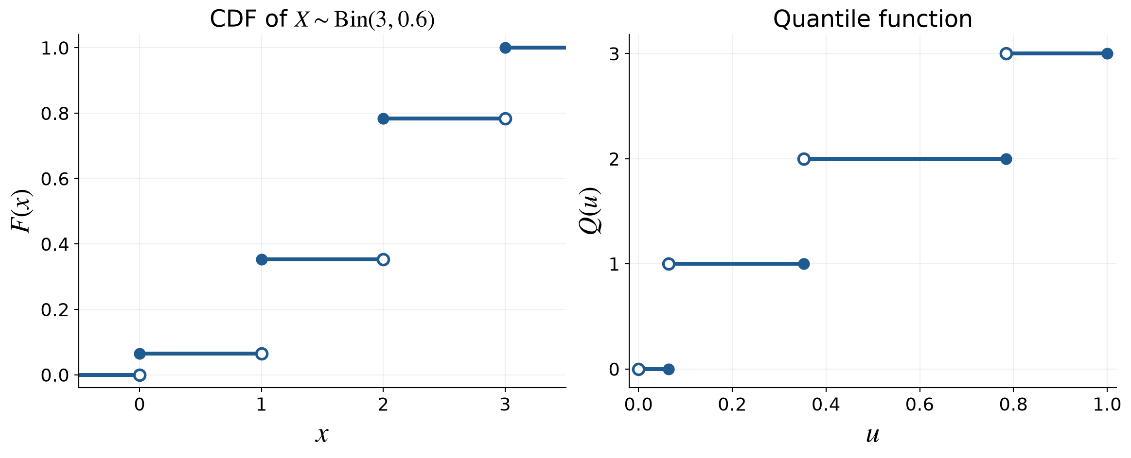
Suppose \(X\sim\Bin(3,0.6)\)

\(x\)	\(0\)	\(1\)	\(2\)	\(3\)
PMF \(\varrho_X(x)\)	\(0.4^3\) \(=0.064\)	\(3(0.6)(0.4^2)\) \(=0.288\)	\(3(0.6^2)(0.4)\) \(=0.432\)	\(0.6^3\) \(=0.216\)
\(x\in\)	\([0,1)\)	\([1,2)\)	\([2,3)\)	\([3,\infty)\)
CDF \(F(x)\)	\(0.064\)	\(0.352\)	\(0.784\)	\(1\)
\(u\in\)	\((0,0.064]\)	\((0.064,0.352]\)	\((0.352,0.784]\)	\((0.784,1]\)
Quantile \(Q(u)\)	\(0\)	\(1\)	\(2\)	\(3\)

E.g., \(U_0=0.63\), \(U_1=0.02\), and \(U_2=0.47\) produce \(X_0=2\), \(X_1=0\), and \(X_2=2\)

\(\exstar\) If \(u=0.70\), what value does the inverse transform produce? What about \(u=0.90\)?

\(F\) is right-continuous; \(Q\) is left-continuous

Zero-inflated exponential random numbers

(Quasi-)Random
Number Generation

CDF

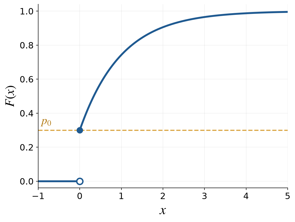
Let \(X\) be nonnegative with

• Probability \(p_0\) of being zero and
• Otherwise an exponential distribution with rate (mean\({}^{-1}\)) \(\lambda\)

\[ \Prob(X=0)=p_0, \qquad X\mid X>0\sim\Exp(\lambda) \]

Its CDF is

\[ F(x)= \begin{cases} 0, & x<0,\\ p_0, & x=0,\\ p_0+(1-p_0)(1-\me^{-\lambda x}), & x>0 \end{cases} \]

For the plot, \(p_0=0.3\) and \(\lambda=1\)

Quantile

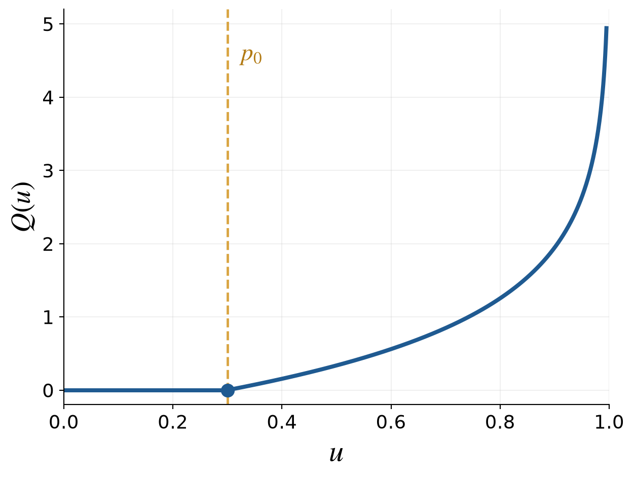
Inverting the CDF gives

\[ Q(u)= \begin{cases} 0, & 0<u\le p_0,\\[0.4em] -\dfrac{1}{\lambda}\log\!\left(\dfrac{1-u}{1-p_0}\right), & p_0<u<1 \end{cases} \]

\(\exstar\) Verify that \(F\{Q(u)\}\ge u\) and identify where equality fails

For the plot, \(p_0=0.3\) and \(\lambda=1\)

An alternative transform

\(\exstar\) Define \(T(u):=Q(1-u)\). Simplify \(T\) and explain why \(T(U)\) has the desired distribution for \(U\sim\Unif(0,1)\) even though \(T\) is not the quantile function. Why might \(T\) be preferred to \(Q\)?

The generalized inverse handles atoms and continuous pieces with one definition

Gaussian mixture random numbers

(Quasi-)Random
Number Generation

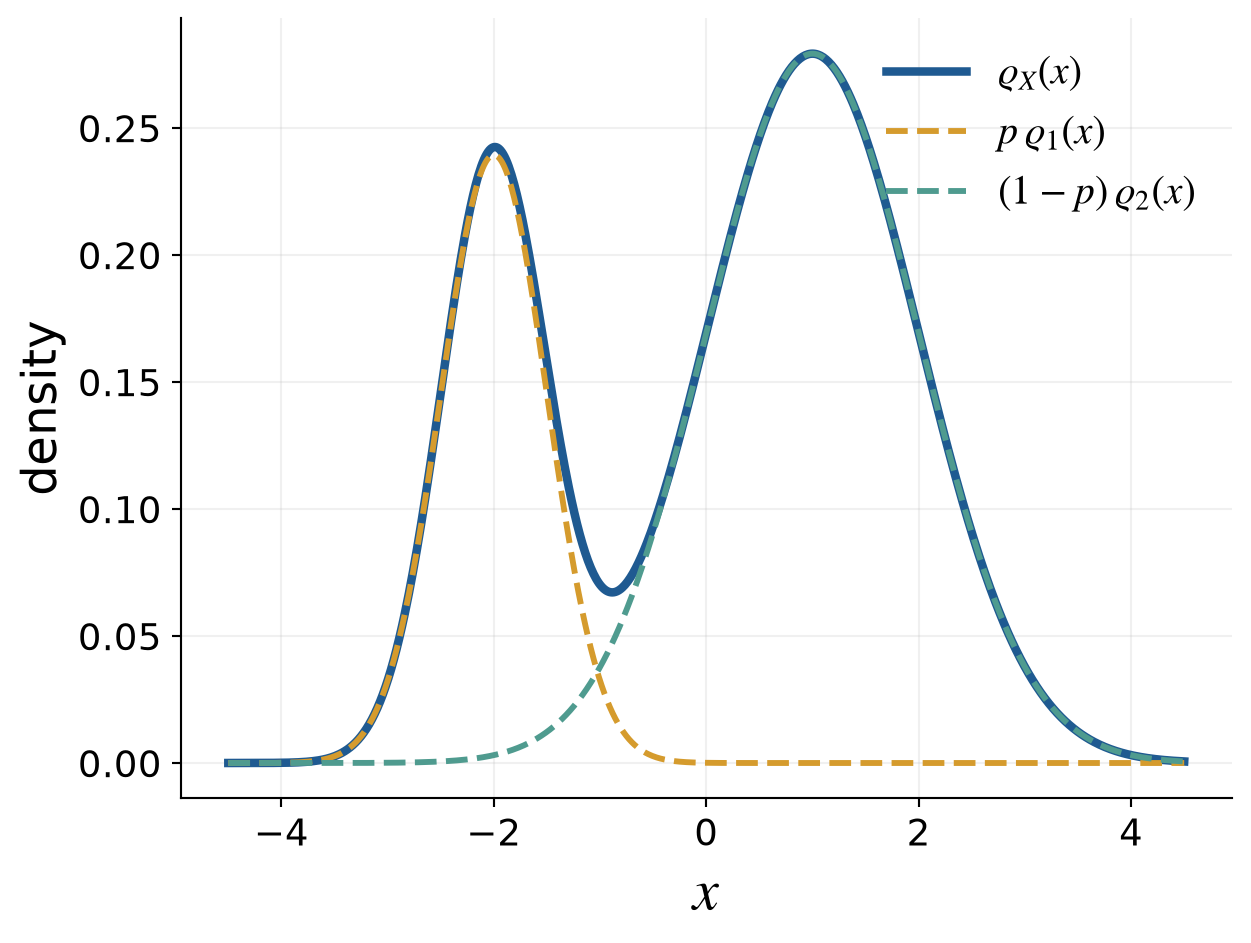
Let the one-dimensional target be a Gaussian mixture:

\[ X\sim p\Norm(\mu_1,\sigma_1^2)+(1-p)\Norm(\mu_2,\sigma_2^2), \qquad 0<p<1 \]

Writing \(\phi\) and \(\Phi\) for the standard normal PDF and CDF,

\[\begin{align*} \varrho_X(x) &=\frac{p}{\sigma_1}\phi\!\left(\frac{x-\mu_1}{\sigma_1}\right) +\frac{1-p}{\sigma_2}\phi\!\left(\frac{x-\mu_2}{\sigma_2}\right),\\ F_X(x) &=p\Phi\!\left(\frac{x-\mu_1}{\sigma_1}\right) +(1-p)\Phi\!\left(\frac{x-\mu_2}{\sigma_2}\right) \end{align*}\]

The PDF and CDF have analytic formulas, but the mixture quantile \(Q=F_X^{-1}\) generally has no analytic closed form

Sampling without the mixture quantile

Numerically inverting \(F_X\) would work, but a hierarchical construction avoids solving \(F_X(x)=u\)

Generate \(U_1,U_2\ \IIDsim\ \Unif(0,1)\) and define

\[ C=\begin{cases}1,&U_1\le p,\\2,&U_1>p,\end{cases} \qquad X=\mu_C+\sigma_C\Phi^{-1}(U_2) \]

Then \(\Prob(C=1)=p\) and \(X\mid C=k\sim\Norm(\mu_k,\sigma_k^2)\)

A mixture chains a discrete component choice with a within-component transform

A concrete mixture

Take

\[\begin{align*} p&=0.3,\\ (\mu_1,\sigma_1)&=(-2,0.5),\\ (\mu_2,\sigma_2)&=(1,1) \end{align*}\]

For \(U_1=0.24\) and \(U_2=0.90\),

\[\begin{align*} C&=1,\\ X&=-2+0.5\Phi^{-1}(0.90)\\ &\approx -1.36 \end{align*}\]

\(\exstar\) Use \(U_1=0.70\) and \(U_2=0.25\). Which component is selected, and what value of \(X\) is generated?

Random Vectors and Stochastic Processes

(Quasi-)Random
Number Generation

• Independent marginals
• Multivariate normal sampling
• Cholesky factorization
• Gaussian processes
• Brownian motion
• Geometric Brownian motion
• Option payoffs and prices

Independent marginals

(Quasi-)Random
Number Generation

For \(\vX=(X_1,\ldots,X_d)\) with independent marginals

\[ \vX=\bigl(Q_1(U_1),\ldots,Q_d(U_d)\bigr), \qquad \vU\sim\Unif[0,1]^d \]

where \(Q_j\) is the quantile function of \(X_j\)

Store \(n\) sampled vectors as an \(n\times d\) array:

\[ \mX= \begin{pmatrix} X_{11} & X_{12} & \cdots & X_{1d}\\ \vdots & \vdots & & \vdots\\ X_{n1} & X_{n2} & \cdots & X_{nd} \end{pmatrix} \]

Rows are samples; columns are coordinates

Multivariate normal sampling

(Quasi-)Random
Number Generation

Let \(\vZ\sim\Norm(\vzero,\mI_d)\) be a column vector of \(d\) independent standard normal random variables, so

\[ \Ex(\vZ)=\vzero, \qquad \Ex(\vZ\vZ^\mathsf{T})=\mI_d \]

Define \(\vX=\mA\vZ+\vmu\). Then

\[\begin{align*} \Ex(\vX) &= \vmu,\\ \cov(\vX) &= \Ex\bigl[(\vX-\vmu)(\vX-\vmu)^\mathsf{T}\bigr] =\Ex(\mA\vZ\vZ^\mathsf{T}\mA^\mathsf{T})\\ &=\mA\Ex(\vZ\vZ^\mathsf{T})\mA^\mathsf{T} =\mA\mA^\mathsf{T} \end{align*}\]

Every linear combination of the components of \(\vX\) is normal. Therefore, if \(\mSigma=\mA\mA^\mathsf{T}\),

\[ \vX=\mA\vZ+\vmu\sim\Norm(\vmu,\mSigma) \]

Cholesky factorization

(Quasi-)Random
Number Generation

Concrete example

For symmetric positive-definite \(\mSigma\), Cholesky factorization gives a lower-triangular \(\mA\) such that \(\mSigma=\mA\mA^\mathsf{T}\)

For

\[ \mSigma=\begin{pmatrix}3&-1\\-1&1\end{pmatrix}, \qquad \mA=\begin{pmatrix}a_{11}&0\\a_{21}&a_{22}\end{pmatrix} \]

matching the entries of \(\mSigma=\mA\mA^\mathsf{T}\) gives

\[\begin{align*} a_{11}^2&=3, &a_{11}a_{21}&=-1, &a_{21}^2+a_{22}^2&=1 \end{align*}\]

Hence

\[ a_{11}=\sqrt3, \qquad a_{21}=-\frac1{\sqrt3}, \qquad a_{22}=\sqrt{\frac23}, \qquad \mA=\begin{pmatrix}\sqrt3&0\\-1/\sqrt3&\sqrt{2/3}\end{pmatrix} \]

General \(2\times2\) covariance

For

\[ \mSigma= \begin{pmatrix} \sigma_1^2 & \rho\sigma_1\sigma_2\\ \rho\sigma_1\sigma_2 & \sigma_2^2 \end{pmatrix}, \qquad \mA= \begin{pmatrix} \sigma_1 & 0\\ \rho\sigma_2 & \sigma_2\sqrt{1-\rho^2} \end{pmatrix} \]

Different factorizations generate the same distribution but may behave differently under low discrepancy sampling

Gaussian processes

Probability

A Gaussian process is a random function whose values at any finite collection of inputs form a multivariate normal random vector

\[ g\sim\GP(\mu,K) \]

means

\[\begin{align*} \Ex[g(t)] &= \mu(t),\\ \Ex\bigl[\{g(t)-\mu(t)\}\{g(x)-\mu(x)\}\bigr] &= K(t,x) \end{align*}\]

For inputs \(t_1,\ldots,t_d\)

\[ \bigl(g(t_1),\ldots,g(t_d)\bigr)^\mathsf{T} \sim\Norm(\vmu,\mSigma), \qquad \Sigma_{jk}=K(t_j,t_k) \]

Brownian motion

Probability

Definition

Brownian motion \(B\) is the Gaussian process with

\[ \mu(t)=0, \qquad K(t,x)=\min(t,x), \qquad t,x\ge0 \]

For \(0=t_0<t_1<\cdots<t_d\)

\[ \bigl(B(t_1),\ldots,B(t_d)\bigr)^\mathsf{T} \sim\Norm(\vzero,\mSigma), \qquad \Sigma_{jk}=\min(t_j,t_k) \]

The covariance structure implies independent normal increments

Covariance matrix and Cholesky factor

For \(0<t_1<t_2<t_3\), let \(\Delta t_1=t_1\) and \(\Delta t_j=t_j-t_{j-1}\). Then

\[ \mSigma= \begin{pmatrix} t_1&t_1&t_1\\ t_1&t_2&t_2\\ t_1&t_2&t_3 \end{pmatrix}, \qquad \mA= \begin{pmatrix} \sqrt{\Delta t_1}&0&0\\ \sqrt{\Delta t_1}&\sqrt{\Delta t_2}&0\\ \sqrt{\Delta t_1}&\sqrt{\Delta t_2}&\sqrt{\Delta t_3} \end{pmatrix}, \qquad \mSigma=\mA\mA^\mathsf{T} \]

Each entry sums the increments shared by both times:

\[ (\mA\mA^\mathsf{T})_{jk} =\sum_{\ell=1}^{\min(j,k)}\Delta t_\ell =t_{\min(j,k)} \]

In general, \(A_{jk}=\sqrt{\Delta t_k}\) for \(k\le j\) and \(A_{jk}=0\) otherwise

Sampling

Let \(Z_1,\ldots,Z_d\ \IIDsim\ \Norm(0,1)\) and start from \(B(t_0)=0\)

\[ B(t_j)=B(t_{j-1})+\sqrt{t_j-t_{j-1}}\,Z_j, \qquad j=1,\ldots,d \]

Equivalently

\[ B(t_j)=\sum_{k=1}^j\sqrt{t_k-t_{k-1}}\,Z_k \]

The Cholesky construction is the familiar cumulative-sum construction for Brownian motion

Geometric Brownian motion

Probability

For \(S_0>0\), drift \(\gamma\), and volatility \(\sigma>0\), define

\[ S(t)=S_0\exp\!\left[ \left(\gamma-\frac{\sigma^2}{2}\right)t+\sigma B(t) \right] \]

Then \(S(t)>0\), its multiplicative increments are lognormal, and

\[ \Ex[S(t)]=S_0\me^{\gamma t} \]

The correction \(-\sigma^2/2\) makes \(\gamma\) the mean growth rate rather than the median growth rate

Risk-neutral asset-price paths

For a non-dividend-paying asset, the risk-neutral model sets \(\gamma=r\)

On \(0=t_0<t_1<\cdots<t_d=T\), define \(\Delta t_j:=t_j-t_{j-1}\). For \(Z_1,\ldots,Z_d\ \IIDsim\ \Norm(0,1)\),

\[ S_j=S_{j-1}\exp\!\left[ \left(r-\frac{\sigma^2}{2}\right)\Delta t_j +\sigma\sqrt{\Delta t_j}\,Z_j \right], \qquad j=1,\ldots,d \]

For equally spaced monitoring times, \(\Delta t_j=T/d\)

The simulated vector \((S_1,\ldots,S_d)\) is the discrete asset path used to evaluate option payoffs

Option payoffs and prices

Quantitative
Finance

The fair price is the expected discounted payoff

\[ \mu=\Ex(\text{discounted payoff}) \]

\[\begin{align*} K &= \text{the }\alert{\text{strike price}}, & T &= \text{the }\alert{\text{time to maturity}},\\ t_j &= jT/d, & S_j &= S(t_j), \qquad j=0,\ldots,d \end{align*}\]

Contract	Discounted payoff
European call	\(\me^{-rT}\max\{S_d-K,0\}\)
European put	\(\me^{-rT}\max\{K-S_d,0\}\)
Arithmetic Asian call	\(\displaystyle \me^{-rT}\max\left\{\frac1T\int_0^T S(t)\,\dif t-K,0\right\}\approx \me^{-rT}\max\{A_d-K,0\}\)

QMCPy FinancialOption offers the right and trapezoidal rules:

\[ \begin{aligned} A_d^{\mathrm{right}} &=\frac1d\sum_{j=1}^d S_j, & A_d^{\mathrm{trap}} &=\frac1d\left(\frac{S_0}{2}+\sum_{j=1}^{d-1}S_j+\frac{S_d}{2}\right) \end{aligned} \]

Path-dependent contracts

Asian, lookback, and barrier payoffs depend on the monitored path, not only the terminal price \(S_d\)

At the monitoring times define

\[ m_d:=\min_{0\le j\le d}S_j, \qquad M_d:=\max_{0\le j\le d}S_j \]

For a barrier \(B\), let \(\mathcal A_B\) be the event that the discretely monitored path activates the option

QMCPy takes \(S_0<B\) for an up barrier and \(S_0>B\) for a down barrier

\[ \begin{array}{ll} \text{up-in}: \mathcal A_B=\{M_d\ge B\}, & \text{up-out}: \mathcal A_B=\{M_d<B\},\\ \text{down-in}: \mathcal A_B=\{m_d\le B\}, & \text{down-out}: \mathcal A_B=\{m_d>B\} \end{array} \]

Lookback and barrier payoffs

Using \(m_d\), \(M_d\), and \(\mathcal A_B\) from the preceding slide:

Contract	Discounted payoff
Lookback call	\(\me^{-rT}(S_d-m_d)\)
Lookback put	\(\me^{-rT}(M_d-S_d)\)
Barrier call	\(\me^{-rT}\max\{S_d-K,0\}\indic(\mathcal A_B)\)
Barrier put	\(\me^{-rT}\max\{K-S_d,0\}\indic(\mathcal A_B)\)

American put: optimal stopping

At the exercise times \(t_0,\ldots,t_d\), the holder chooses a stopping index \(J\) using only prices observed through \(t_J\)

Let \(\mathcal T_d\) be the set of these stopping indices. The fair price is

\[ \mu_{\mathrm{AmPut}} =\sup_{J\in\mathcal T_d} \Ex\!\left[ \me^{-rt_J}\max\{K-S_J,0\} \right] \]

• A European put restricts exercise to \(J=d\)
• An American put may exercise earlier when doing so is more valuable
• With no dividends and \(r\ge0\), early exercise does not improve an American call, so we omit it here

Low Discrepancy Sampling

Low
Discrepancy

Discrepancy
Measures

• What does low discrepancy mean?
• Low discrepancy sequences
• Bias–variance decomposition
• Shrinkage estimators
• Transport maps and normalizing flows

What does low discrepancy mean?

Low
Discrepancy

Discrepancy
Measures

Relaxing the requirement that \(\vU_0,\ldots,\vU_{n-1}\) be IID allows carefully constructed samples to cover \([0,1]^d\) more evenly

\[ \vU_0,\ldots,\vU_{n-1}\ \LDsim\ \Unif[0,1]^d \]

The empirical distribution of the sample is close to the uniform distribution

Discrepancy quantifies that difference; precise definitions come later

Low discrepancy replaces independent placement by deliberate coverage

Low discrepancy sequences

Low
Discrepancy

Discrepancy
Measures

Important families include

• digital sequences, especially Sobol’ sequences
• lattice sequences
• Halton sequences
• Kronecker sequences

They are available in deterministic and randomized forms through SciPy and QMCPy

In software arrays rows correspond to samples and columns to coordinates

Bias–variance decomposition

Statistics

Estimation

Recall the bias–variance decomposition from Deck 01: for an estimator \(\Theta\) of \(\theta\),

\[\begin{align*} \mse(\Theta) &=\Ex[(\Theta-\theta)^2]\\ &=[\bias(\Theta)]^2+\var(\Theta) \end{align*}\]

The identity is unchanged; the source of randomness changes:

• An IID sample-mean estimator is unbiased and has positive variance
• A deterministic low discrepancy estimator has no sampling variance, but its deterministic error may be nonzero
• A randomized low discrepancy estimator has a sampling distribution, enabling variance estimation while retaining improved space filling

Shrinkage estimators

Statistics

Estimation

Suppose \(Y_0,\ldots,Y_{n-1}\ \IIDsim\ Y\), where

\[ \Ex(Y)=\mu, \qquad \var(Y)=\sigma^2, \qquad \hmu_n=\frac1n\sum_{i=0}^{n-1}Y_i \]

For the estimator \(\alpha\hmu_n\)

\[ \mse(\alpha\hmu_n) =(1-\alpha)^2\mu^2+\alpha^2\frac{\sigma^2}{n} \]

\(\exstar\) Find the value of \(\alpha\) that minimizes this MSE. Is the minimizing estimator unbiased?

Transport maps and normalizing flows

(Quasi-)Random
Number Generation

The quantile transform is a one-dimensional transport. In \(d\) dimensions, start with an easy reference density \(\varrho_0\) and an invertible, differentiable map \(T:\reals^d\to\reals^d\):

\[ \vZ\sim\varrho_0, \qquad \vX=T(\vZ) \]

The change-of-variables formula gives

\[ \varrho_X(\vx) =\varrho_0\!\left(T^{-1}(\vx)\right) \left|\det \nabla T^{-1}(\vx)\right| \]

A normalizing flow composes manageable maps \(T=T_m\circ\cdots\circ T_1\), often tuning their parameters to fit a target

A transport moves every sample and keeps equal weights; importance sampling keeps proposal samples and assigns unequal weights

A triangular flow creates curved dependence

Let \(Z_1,Z_2\ \IIDsim\ \Norm(0,1)\) and, for \(b>0\), define

\[ X_1=Z_1, \qquad X_2=Z_2+b(Z_1^2-1) \]

This nonlinear map is easy to invert and has a simple Jacobian:

\[ T_b^{-1}(\vx) =\begin{pmatrix}x_1\\x_2-b(x_1^2-1)\end{pmatrix}, \qquad \nabla T_b(\vz) =\begin{pmatrix}1&0\\2bz_1&1\end{pmatrix}, \qquad \det\nabla T_b=1 \]

Thus, with \(\phi\) the standard normal density,

\[ \varrho_X(x_1,x_2) =\phi(x_1)\phi\!\left(x_2-b(x_1^2-1)\right), \qquad \Ex(X_2\mid X_1=x_1)=b(x_1^2-1) \]

One layer turns independent Gaussian coordinates into a curved, dependent target. If no useful invertible map is available, acceptance–rejection offers another route from an easy proposal to the target

Acceptance–Rejection Sampling

(Quasi-)Random
Number Generation

• The acceptance–rejection algorithm
• Why acceptance–rejection works
• Efficiency and method comparison

The acceptance–rejection algorithm

(Quasi-)Random
Number Generation

Suppose

• Proposal distribution: \(Z\) is easy to sample with density \(\varrho_Z\)
• Target distribution: density \(c\varrho\), with known \(\varrho\) and possibly unknown \(c>0\)
• \(\varrho(x)\le M\varrho_Z(x)\) for all \(x\)

Repeat until a proposal is accepted:

1. Generate \(Z\sim\varrho_Z\) and \(U\sim\Unif[0,1]\) independently

2. Accept \(Z\) as \(X\) if

   \[ U\le\frac{\varrho(Z)}{M\varrho_Z(Z)} \]

Otherwise reject \(Z\) and try again

Why acceptance–rejection works

(Quasi-)Random
Number Generation

For a small interval \(\dif z\) around \(z\)

\[\begin{align*} \Prob(Z\in\dif z,\text{ accept}) &=\varrho_Z(z)\dif z\, \frac{\varrho(z)}{M\varrho_Z(z)}\\ &=\frac{\varrho(z)}{M}\dif z \end{align*}\]

Conditioning on acceptance gives the target density

\[ \varrho_{Z\mid\text{accept}}(z) =\frac{\varrho(z)/M}{\Prob(\text{accept})} =c\varrho(z), \qquad \Prob(\text{accept})=\frac{1}{Mc} \]

Efficiency and method comparison

Pseudorandom
Numbers

Low
Discrepancy

Obtaining \(n\) accepted samples requires an average of \(nMc\) proposals

Method	Main requirement	Compatible with low discrepancy?
Quantile transform \(X=Q(U)\)	Quantile function \(Q\)	Yes
Normal transform \(\vX=\mA\vZ+\vmu\)	\(\mSigma=\mA\mA^\mathsf{T}\)	Yes
Transport map \(\vX=T(\vZ)\)	Invertible \(T\) and its Jacobian	Yes
Acceptance–rejection	\(\varrho\le M\varrho_Z\)	With care

Choose a proposal distribution close to the target distribution so that \(Mc\) is near one

Big Ideas

Probability

Statistics

Estimation

• Start with uniform samples and transform them to the desired distribution
• The generalized inverse works for discrete and continuous distributions
• Mixtures combine a discrete component choice with a conditional transform
• Independent marginal transforms do not create dependence; correlated normal vectors require a matrix factorization
• Gaussian-process sampling reduces finite collections of function values to multivariate normal sampling
• Low discrepancy points trade independent placement for more even coverage
• Bias and variance are distinct contributions to mean squared error
• Acceptance–rejection samples from an unnormalized density when a suitable proposal envelope is available

Companion GeneratingSamples notebook