Variance and variation reduction
Variance
Keep the target quantity, but change its computational representation:
\[\begin{gather*}
\vX\sim\varrho_{\mathrm{tar}},\quad Y=f(\vX),\qquad
\vZ\sim\varrho_{\mathrm{prop}},\quad Y_g=g(\vZ) \\
\alerttext{And} \quad \mu=\Ex(Y) = \Ex(Y_g)
\end{gather*}\]
Two sample means estimate the same \(\mu\) :
\[\begin{align*}
\hmu_{f,n}&=\frac1n\sum_{i=0}^{n-1}f(\vX_i),&
\hmu_{g,n}&=\frac1n\sum_{i=0}^{n-1}g(\vZ_i)
\end{align*}\]
Change the function, the sampling distribution, or both
Seek lower error for comparable computational work
Changing only the function gives the special case \(g(\vX)\)
Label contributions by method: \(Y_{\mathrm{IS}}\) , \(Y_{\mathrm{CV}}\) , \(Y_{\mathrm{CMC}}\)
Variance reduction
For IID samples and finite second moments, both sample means are unbiased:
\[\begin{align*}
\var(\hmu_{f,n})&=\frac{\var_{\mathrm{tar}}\{f(\vX)\}}n,&
\var(\hmu_{g,n})&=\frac{\var_{\mathrm{prop}}\{g(\vZ)\}}n
\end{align*}\]
Their MSEs equal their variances; IID RMSE is \(\Order(n^{-1/2})\)
Equal means allow different output distributions and different variances
For randomized low discrepancy inputs, dependence changes the variance formula
The two methods need not be independent of one another for these individual variance formulas. Each method needs independent replicates internally. Compare computational costs as well as the variance of one contribution. Introduction showed that accepting some bias can reduce MSE; here we compare unbiased estimators. Degenerate zero-variance cases need no asymptotic rate.
Variation reduction for low discrepancy sampling
To compare designs on the unit cube, make the uniform inputs explicit:
\[\begin{align*}
\vX&=\vT(\vU),& h_f(\vu)&=f\bigl(\vT(\vu)\bigr),\\
\vZ&=\vS(\vU),& h_g(\vu)&=g\bigl(\vS(\vu)\bigr)
\end{align*}\]
Both cube integrands have integral \(\mu\) ; keep the nodes \(\vu_0,\ldots,\vu_{n-1}\) fixed
For \(h_g\in\mathcal H_K\) and uniform distribution \(F_{\mathrm{unif}}\) ,
\[
\left|\mu-\frac1n\sum_{i=0}^{n-1}h_g(\vu_i)\right|
\le D\bigl(\{\vu_i\}_{i=0}^{n-1},F_{\mathrm{unif}};K\bigr)\norm{h_g}_{\mathcal H_K}
\]
Nodes determine discrepancy ; the composed cube integrand determines variation
Seek a smaller \(\norm{h_g}_{\mathcal H_K}\) for the same nodes and kernel
The notation \(\vT\) identifies a transport from uniform inputs to the target; \(\vS\) generates proposal draws. Neither map must be displayed when uniform inputs are incidental. This common-cube comparison assumes compatible input dimensions; conditioning can reduce dimension. The bound is the Markov Chain Monte Carlo worst-case integration-error bound. For sufficiently smooth composed cube integrands, nested uniform scrambling gives variance nearly \(\Order(n^{-3})\) and RMSE nearly \(\Order(n^{-3/2})\) . This is not a guarantee for every randomization or integrand. Owen (1997) provides the variance result.
The Keister example
Write the original integral as a target expectation :
\[\begin{gather*}
\mu=\int_{\reals^d}\cos(\norm{\vx})\me^{-\norm{\vx}^2}\,\dif\vx
=\Ex_{\mathrm{tar}}[f(\vX)],\\
\vX\sim\Norm(\vzero,\mI_d/2),\qquad
f(\vx)=\mpi^{d/2}\cos(\norm{\vx})
\end{gather*}\]
Choose \(\vZ_a\sim\Norm(\vzero,\mI_d/a^2)\) and apply a density correction :
\[
g_a(\vz)=\frac{(2\mpi)^{d/2}}{a^d}
\cos(\norm{\vz})\exp\bigl[-(1-a^2/2)\norm{\vz}^2\bigr]
\]
Every \(a>0\) gives \(\Ex[g_a(\vZ_a)]=\mu\) ; changing \(a\) changes the contribution
First identify a probability density in the original integral. Here \(\varrho_{\mathrm{tar}}(\vx)=\mpi^{-d/2}\me^{-\norm{\vx}^2}\) is the \(\Norm(\vzero,\mI_d/2)\) density, so \(\me^{-\norm{\vx}^2}=\mpi^{d/2}\varrho_{\mathrm{tar}}(\vx)\) . The factor \(\mpi^{d/2}\) belongs in \(f\) when the integral is written as \(\Ex_{\mathrm{tar}}[f(\vX)]\) .
Keister on the unit cube
Set \(\vS_a(\vu)=\bigl(\Phi^{-1}(u_j)/a\bigr)_{j=1}^d\) and \(h_a(\vu)=g_a\bigl(\vS_a(\vu)\bigr)\)
With \(\vq(\vu)=\bigl(\Phi^{-1}(u_j)\bigr)_{j=1}^d\) ,
\[
h_a(\vu)=\frac{(2\mpi)^{d/2}}{a^d}
\cos\bigl(\norm{\vq(\vu)}/a\bigr)
\exp\bigl[-(2-a^2)\norm{\vq(\vu)}^2/(2a^2)\bigr]
\]
\(\exstar\) Verify \(g_a=f\varrho_{\mathrm{tar}}/\varrho_{\mathrm{prop},a}\) and \(\int_{[0,1]^d}h_a(\vu)\,\dif\vu=\mu\)
\(0<a^2\le2\) : \(h_a\) is bounded ; \(a=\sqrt2\) gives \(g_a=f\) \(2<a^2<4\) : \(h_a\) is unbounded but has finite variance, including \(a=1.6\) \(a^2\ge4\) : infinite variance
Choose \(a\) by estimator variance or cube-integrand variation
Every positive \(a\) preserves the mean. The second moment is \[
\Ex[g_a(\vZ_a)^2]=\frac{(2\mpi)^{d/2}}{a^d}
\int_{\reals^d}\cos^2(\norm{\vz})
\exp\bigl[-(2-a^2/2)\norm{\vz}^2\bigr]\,\dif\vz.
\] It is finite precisely when \(a^2<4\) . For \(2<a^2<4\) , the cube-boundary singularity is mild enough for square integrability. At \(a^2=4\) , Gaussian decay disappears and the squared cosine cannot provide cancellation; for larger \(a^2\) , the envelope grows. The notebook uses \(a=1.6\) to explore an unbounded integrand that still has finite variance.
Explore \(a\) in the Keister notebook
An exact transport \(\vT:\mathcal Z\to\mathcal X\) satisfies
\[
\varrho_{\mathrm{tar}}\bigl(\vT(\vz)\bigr)
\left|\det\nabla\vT(\vz)\right|
=\varrho_{\mathrm{prop}}(\vz)
\]
Then \(w_T(\vz)=1\) wherever \(\varrho_{\mathrm{prop}}(\vz)>0\) , and so \(\vX=\vT(\vZ)\sim\varrho_{\mathrm{tar}}\) , and
\[
g(\vz)=f\bigl(\vT(\vz)\bigr),\qquad
g(\vZ)\stackrel d=f(\vX)
\]
Exact transport preserves the whole output distribution , including IID variance
Provides access to target samples; construction and evaluation costs can differ
Different transports can change low discrepancy performance through the cube integrand
Exact transport makes importance weights constant
Exact transport \(\vT\)
\(w_T(\vz)=1\) \(f\bigl(\vT(\vZ)\bigr)\)
Identity map \(\vT(\vz)=\vz\)
\(w(\vz)=\varrho_{\mathrm{tar}}(\vz)/\varrho_{\mathrm{prop}}(\vz)\) \(f(\vZ)w(\vZ)\)
Exact transport changes samples ; importance sampling changes contributions
Same expectation \(\Ex_{\mathrm{tar}}[f(\vX)]=\Ex_{\mathrm{prop}}[g(\vZ)]=\mu\)
but output distributions and variances may differ (want them to)
Importance sampling
Importance
Choose \(\varrho_{\mathrm{prop}}>0\) wherever \(f\varrho_{\mathrm{tar}}\ne0\)
\[\begin{align*}
w(\vz)&=\frac{\varrho_{\mathrm{tar}}(\vz)}{\varrho_{\mathrm{prop}}(\vz)},&
g(\vz)&=f(\vz)w(\vz),\\
\mu&=\Ex_{\mathrm{tar}}[f(\vX)]
=\Ex_{\mathrm{prop}}[g(\vZ)]
\end{align*}\]
For \(\vZ_0,\ldots,\vZ_{n-1}\ \IIDsim\ \varrho_{\mathrm{prop}}\) ,
\[
Y_{\mathrm{IS}}=g(\vZ)=f(\vZ)w(\vZ),\qquad \Ex(Y_{\mathrm{IS}})=\mu
\]
\[
\hmu_{\mathrm{IS},n}=\frac1n\sum_{i=0}^{n-1}Y_{\mathrm{IS},i}
=\frac1n\sum_{i=0}^{n-1}f(\vZ_i)w(\vZ_i)
\]
\(w\) is the weight function; \(W=w(\vZ)\) is its random value
Weighted empirical distributions
As in Markov Chain Monte Carlo: empirical distributions , put mass at each sample point
For \(\vZ_i\ \IIDsim\ F_{\mathrm{prop}}\) , require \(\varrho_{\mathrm{prop}}>0\) wherever \(\varrho_{\mathrm{tar}}>0\)
\[\begin{align*}
\widehat F_{n,w}
&=\frac{\sum_{i=0}^{n-1}w(\vZ_i)\,\delta_{\vZ_i}}
{\sum_{i=0}^{n-1}w(\vZ_i)},
& w(\vz)&=\frac{\varrho_{\mathrm{tar}}(\vz)}{\varrho_{\mathrm{prop}}(\vz)},\\
\int f(\vx)\,\dif\widehat F_{n,w}(\vx)
&=\frac{\sum_{i=0}^{n-1}w(\vZ_i)f(\vZ_i)}
{\sum_{i=0}^{n-1}w(\vZ_i)}
& &\xrightarrow[n\to\infty]{\mathrm{a.s.}}\mu
\end{align*}\]
Normalized weights sum to one; require a positive denominator\(\widehat F_{n,w} \approx F_{\mathrm{tar}}\) ; generally different at finite \(n\) Self-normalized estimates: consistent, generally biased at finite \(n\)
Use the same \(\widehat F_n\) and point-mass \(\delta_{\vx_i}\) notation as the empirical-distribution development in Markov Chain Monte Carlo, with the subscript \(w\) recording the weights. The points still have the proposal law; weighting changes their empirical masses, not their locations or sampling law. The almost-sure limit assumes IID proposal draws, normalized target and proposal densities, target-support coverage, and \(\Ex_{\mathrm{tar}}|f(\vX)|<\infty\) . The denominator can be zero at finite \(n\) if every sampled weight is zero.
Without self-normalization, the weighted empirical measure is \[\begin{align*}
\widehat M_{n,w}&=\frac1n\sum_{i=0}^{n-1}w(\vZ_i)\delta_{\vZ_i},\\
\int f(\vx)\,\dif\widehat M_{n,w}(\vx)&=\hmu_{\mathrm{IS},n},&
\Ex[\widehat M_{n,w}(A)]&=F_{\mathrm{tar}}(A)
\end{align*}\] for measurable sets \(A\) . Its total mass \(n^{-1}\sum_i w(\vZ_i)\) has expectation one, but generally is not exactly one, so it need not be a probability measure. Ordinary importance sampling is unbiased for integrable \(f\) ; self-normalization produces a probability measure but generally loses finite-sample unbiasedness. Full support coverage is needed to approximate the whole target distribution, which is stronger than covering only the support of \(f\varrho_{\mathrm{tar}}\) for one particular integral. A weighted empirical approximation to the target also does not imply that the scalar importance contribution \(f(\vZ)w(\vZ)\) has the same distribution as \(f(\vX)\) .
One proposal, three unbiased estimators
\[\begin{gather*}
\varrho_{\mathrm{prop}}(z)=1,\qquad
\varrho_{\mathrm{tar}}(x)=2x,\qquad 0<x,z<1,\\
Z_0,\ldots,Z_{n-1}\ \IIDsim\ \Unif(0,1),\qquad
\mu=\Ex_{\mathrm{tar}}[f(X)]
\end{gather*}\]
Construction
\(T(z)=\sqrt z\) \(w(z)=2z\) Accept \(X=Z\) if \(V\le Z\)
Contribution
\(f(\sqrt Z)\) \(2Zf(Z)\) \(f(X)\) for accepted \(X\)
Estimator
\(\displaystyle\frac1n\sum_{i=0}^{n-1}f(\sqrt{Z_i})\) \(\displaystyle\frac1n\sum_{i=0}^{n-1}2Z_if(Z_i)\) \(\displaystyle\frac1n\sum_{i=0}^{n-1}f(X_i)\)
Output distribution
Same as \(Y=f(X)\)
Generally different from \(Y\)
Same as \(Y=f(X)\)
Proposal cost
\(n\) \(n\) Average \(2n\) for \(n\) accepted
Acceptance–rejection: independent \(V\sim\Unif(0,1)\) for each proposal; continue until \(n\) accepted points \(X_0,\ldots,X_{n-1}\)
All three estimates are unbiased for the same target expectation when \(f\) is integrable. The acceptance–rejection column links to the matching triangular target example in Generating Samples. Its envelope constant is \(M=2\) , so the acceptance probability is \(1/2\) . Accepted points are indexed separately from the proposal stream; continue drawing fresh independent proposal/decision pairs until exactly \(n\) acceptances have been collected. The number of proposals is random, with mean \(2n\) . The other two columns use exactly \(n\) proposals. Thus equal numbers of averaged contributions do not mean equal proposal costs. Each rejection attempt also requires an independent decision uniform \(V\) . The acceptance–rejection estimator here averages a fixed number of accepted points, not a random number obtained from a fixed proposal budget.
Seeing the contribution variances
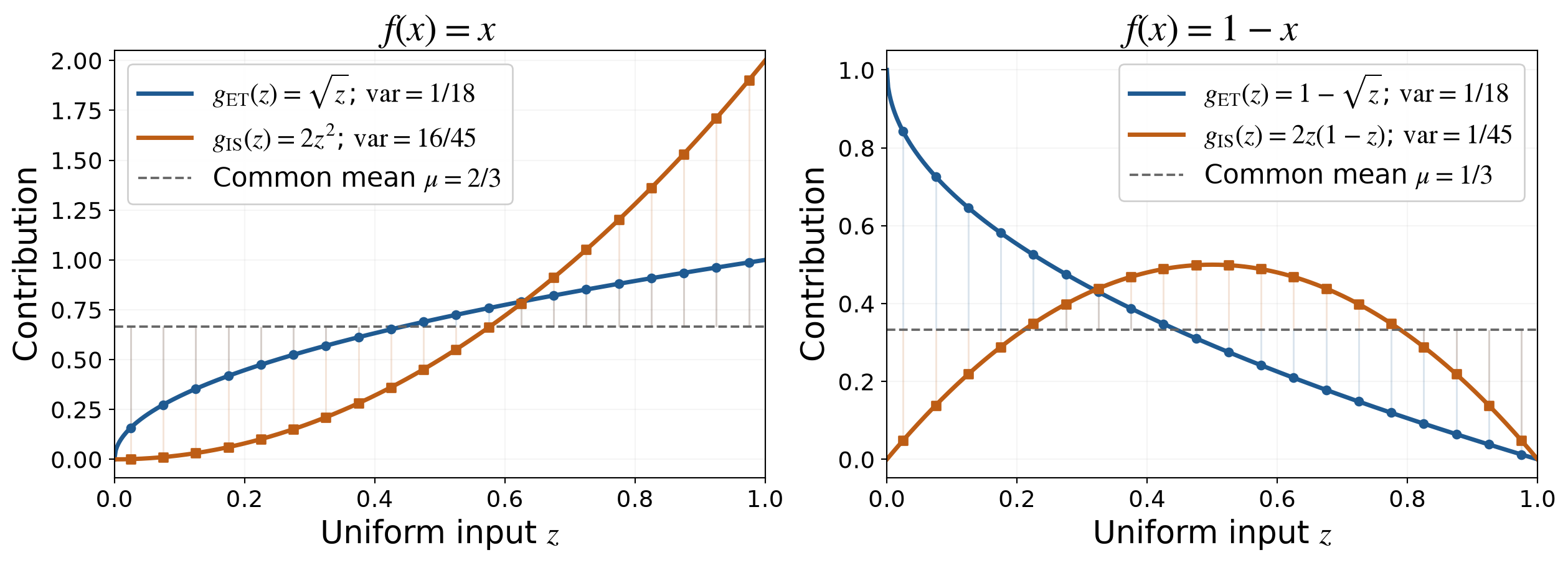
\(g_{\mathrm{ET}}(z)=f(\sqrt z)\) ; \(g_{\mathrm{IS}}(z)=2zf(z)\) ; both use \(Z\sim\Unif(0,1)\)
Markers: equally probable input quantiles; dashed line: common mean
The dots are deterministic quantile illustrations, not a random Monte Carlo sample. For each curve, each marker represents the midpoint of a probability bin of mass 1/20. Both curves use the same uniform input points (i+1/2)/20. Vertical segments show deviations from the mean. Since both inputs are uniform, variance is the integral of the squared vertical deviations. The two curves in each plot share the same axes. For f(x)=x, importance sampling increases contribution variance by a factor 6.4. For f(x)=1-x, it reduces contribution variance by a factor 2.5. The exact-transport output f(sqrt(Z)) has the same distribution as f(X), so the blue curves also represent the target-output variance.
Compare transport and importance sampling
\(Z\sim\Unif(0,1)\) ; target density \(\varrho_{\mathrm{tar}}(x)=2x\) on \((0,1)\)
\[\begin{align*}
Y_T&=f(\sqrt Z),&Y_{\mathrm{IS}}&=2Zf(Z)
\end{align*}\]
\(\exstar\) Compare the two contributions For \(f(x)=x\) , compute their means and variances Repeat for \(f(x)=1-x\) Explain why the variance ranking reverses
For f(x)=x, both means are 2/3; the transport variance is 1/18 and the IS variance is 16/45. For f(x)=1-x, both means are 1/3; the transport variance remains 1/18 and the IS variance is 1/45. Compute each variance as its second moment minus the squared mean. The contribution’s shape, not the target density alone, determines the variance. In the second case, the factor 2Z partly offsets the decrease in 1-Z. The next slide collects the results. These compare equal numbers of contributions, without claiming equal computational cost.
Variance depends on the function
Displayed variances: one estimator contribution
Sample-mean variances: divide by \(n\)
\(x\) \(2/3\) \(1/18\) \(16/45\) transport
\(1-x\) \(1/3\) \(1/18\) \(1/45\) importance sampling
No universal variance winner
Target samples support ordinary averages for every \(f\)
Weighted proposals can be better or worse for a particular \(f\)
Brownian motion with drift
Let \(\vX\sim\Norm(\vzero,\mSigma)\) be the target Brownian path, with \(\Sigma_{jk}=\min(t_j,t_k)\) and discounted payoff \(Y=f(\vX)\)
Choose \(\vZ\sim\Norm(\va,\mSigma)\) , where \(\va=\theta(t_1,\ldots,t_d)^\mathsf T\)
\[\begin{align*}
w(\vz)&=\frac{\varrho_{\mathrm{tar}}(\vz)}{\varrho_{\mathrm{prop}}(\vz)}
=\exp\!\left(-\theta z_d+\frac{\theta^2t_d}{2}\right),\\
Y_{\mathrm{IS}}&=f(\vZ)w(\vZ),\qquad \Ex_{\mathrm{prop}}[Y_{\mathrm{IS}}]=\mu
\end{align*}\]
Drift makes positive payoffs more common
Weights preserve the target expectation; a good drift can reduce variance
Asian option variance-reduction notebook
Control Variates and Conditioning
Variance
Control variates
Variance
Let \(\boldsymbol{\eta}(\vX)=(\eta_1(\vX),\ldots,\eta_m(\vX))^\mathsf T\) have known zero mean
For fixed coefficients \(\vbeta\) , define
\[
Y_{\mathrm{CV}}=g(\vX)=f(\vX)-\vbeta^\mathsf T\boldsymbol{\eta}(\vX)
\]
Then \(\Ex(Y_{\mathrm{CV}})=\Ex[f(\vX)]=\mu\) , so
\[
\hmu_{\mathrm{CV},n}
=\frac1n\sum_{i=0}^{n-1}Y_{\mathrm{CV},i}
\]
is unbiased
Choose \(\vbeta\) to make \(\var(Y_{\mathrm{CV}})\) as small as possible
Optimal coefficients from covariances
\(Y=f(\vX)\) , \(\boldsymbol{\eta}=\boldsymbol{\eta}(\vX)\) , \(\Ex(\boldsymbol{\eta})=\vzero\)
Define the control covariance matrix and response–control covariances:
\[\begin{align*}
\mSigma_\eta&=\cov(\boldsymbol{\eta},\boldsymbol{\eta}),&
(\mSigma_\eta)_{jk}&=\cov(\eta_j,\eta_k),\\
\boldsymbol{\kappa}&=\cov(\boldsymbol{\eta},Y),&
\kappa_j&=\cov\{\eta_j(\vX),f(\vX)\}
\end{align*}\]
Since \(Y_{\mathrm{CV}}-\mu=(Y-\mu)-\vbeta^\mathsf T\boldsymbol{\eta}\) ,
\[\begin{align*}
\var(Y_{\mathrm{CV}})
&=\Ex\bigl[((Y-\mu)-\vbeta^\mathsf T\boldsymbol{\eta})^2\bigr]\\
&=\var(Y)-2\vbeta^\mathsf T\boldsymbol{\kappa}
+\vbeta^\mathsf T\mSigma_\eta\vbeta
\end{align*}\]
The variance is a quadratic function of the coefficients
Minimize the control-variate variance
For nonsingular \(\mSigma_\eta\) , differentiate and set the gradient to zero:
\[\begin{align*}
\nabla_{\vbeta}\var(Y_{\mathrm{CV}})
&=-2\boldsymbol{\kappa}+2\mSigma_\eta\vbeta=\vzero,\\
\mSigma_\eta\vbeta_*&=\boldsymbol{\kappa},\qquad
\vbeta_*=\mSigma_\eta^{-1}\boldsymbol{\kappa}
\end{align*}\]
Completing the square confirms the minimum:
\[\begin{align*}
\var(Y_{\mathrm{CV}})
&=\var(Y)-\boldsymbol{\kappa}^\mathsf T\mSigma_\eta^{-1}\boldsymbol{\kappa}\\
&\quad +(\vbeta-\vbeta_*)^\mathsf T\mSigma_\eta(\vbeta-\vbeta_*)
\end{align*}\]
Minimum variance: \(\var(Y)-\boldsymbol{\kappa}^\mathsf T\mSigma_\eta^{-1}\boldsymbol{\kappa}\)
One control: \(\beta_*=\cov\{f(\vX),\eta_1(\vX)\}/\var\{\eta_1(\vX)\}\)
Assume finite second moments. A nonsingular covariance matrix is positive definite, so the final quadratic term is nonnegative and the minimizer is unique. With redundant controls, the covariance matrix can be singular; remove redundant controls or solve the normal equations with a pseudoinverse. The cross-covariance vector is in the covariance matrix’s range, and the optimal residual is unchanged by coefficient directions in its null space. At the optimum, cov(eta, Y_CV)=kappa-Sigma_eta beta_*=0: the residual is uncorrelated with every control. In practice, solve the covariance system rather than explicitly forming the inverse.
One control: variance and cost
Suppose \(\Ex(\eta)=0\) and
\[
\var(Y)=9,\qquad \var(\eta)=4,\qquad \cov(Y,\eta)=3
\]
\(\exstar\) Use \(Y_{\mathrm{CV}}=Y-\beta\eta\) Find \(\beta_*\) and the minimum contribution variance If a controlled contribution costs twice as much, which method needs less work for the same IID RMSE? Why fit \(\beta\) on an independent pilot?
Ignore setup and pilot cost for the work comparison; assume independent contributions
The optimal coefficient is 3/4, and the minimum variance is 9-3^2/4=27/4=6.75. If a direct contribution costs c, compare 9c with (27/4)(2c)=13.5c. The direct method needs less work for the same IID RMSE, ignoring setup, pilot costs, and integer sample counts. An independent pilot makes the fitted coefficient independent of the main samples. Conditional on the pilot, the control still has mean zero, so the final mean remains unbiased, assuming integrability. Fitting on the main samples does not generally retain exact unbiasedness.
Choosing coefficients by least squares
Center the response and control values:
\[\begin{align*}
y_i&=f(\vx_i),& c_i&=y_i-\overline y,\\
H_{ij}&=\eta_j(\vx_i)-\overline{\eta}_j
\end{align*}\]
Then
\[
\hvbeta=\argmin_{\vb}\norm{\vc-\mH\vb}^2
\]
When \(\mH^\mathsf T\mH\) is nonsingular,
\[
\hvbeta=(\mH^\mathsf T\mH)^{-1}\mH^\mathsf T\vc
\]
Sample covariances: \(\widehat{\mSigma}_\eta=\mH^\mathsf T\mH/(n-1)\) , \(\widehat{\boldsymbol{\kappa}}=\mH^\mathsf T\vc/(n-1)\)
The residual is orthogonal to the column space of \(\mH\)
Use an independent pilot to estimate beta if exact unbiasedness of the final IID estimator is required.
Practical control-variate choices
Good controls are inexpensive , have known means, and are strongly related to \(f\)
More controls can reduce the sample size needed for a target accuracy
Poor controls may increase computation without reducing variance
For IID sampling, least squares targets variance reduction
For low discrepancy sampling, choose coefficients to reduce variation , not sampling variance
A control variate turns known expectations into information about an unknown expectation
Conditional Monte Carlo
Variance
Probability
Let \(V\) be a conditioning variablelaws of total expectation and variance
\[\begin{align*}
\Ex(Y)&=\Ex_V\{\Ex(Y\mid V)\},\\
\var(Y)&=\Ex_V\{\var(Y\mid V)\}+\var_V\{\Ex(Y\mid V)\}
\end{align*}\]
Therefore
\[
\var_V\{\Ex(Y\mid V)\}\le\var(Y)
\]
If \(Y=f(X_1,\ldots,X_d)\) and
\[
Y_{\mathrm{CMC}}=g(\vX_{2:d})=\Ex(Y\mid \vX_{2:d})
\]
is analytic, estimate \(\mu\) by averaging \(Y_{\mathrm{CMC},i}\) instead of \(Y_i\)
Analytically averaging over part of the randomness reduces variance
Conditional density estimation
Write the simulator on uniform inputs as \(Y=h(\vU)\) with \(\vU\sim\Unif[0,1]^d\)
Suppose \(h\) is increasing in \(u_1\) and
\[
y=h(u_1,\vu_{2:d})\iff u_1=g(y;\vu_{2:d})
\]
Extend the inverse by clipping to \([0,1]\) outside the conditional support
\[\begin{align*}
F_{Y\mid \vU_{2:d}}(y\mid \vu_{2:d})
&=\Prob\{U_1\le g(y;\vu_{2:d})\}\\
&=g(y;\vu_{2:d}),\\
\varrho_Y(y)
&=\int_{[0,1]^{d-1}}\frac{\partial g}{\partial y}(y;\vu_{2:d})\,\dif\vu_{2:d}
\end{align*}\]
Thus a density value becomes an expectation of a conditional density
Let
\[
Y=\gamma_1U_1+\cdots+\gamma_dU_d,
\qquad \vU\sim\Unif[0,1]^d,
\qquad \gamma_j>0
\]
Solving for \(u_1\) gives
\[
g(y;\vu_{2:d})=\frac{y-\sum_{j=2}^d\gamma_ju_j}{\gamma_1}
\]
when \(\sum_{j=2}^d\gamma_ju_j\le y\le\gamma_1+\sum_{j=2}^d\gamma_ju_j\)
Hence
\[
\varrho_Y(y)=\Ex\!\left[
\frac1{\gamma_1}\indic\!\left\{
\sum_{j=2}^d\gamma_jU_j\le y\le
\gamma_1+\sum_{j=2}^d\gamma_jU_j
\right\}\right]
\]
Conditional Monte Carlo notebook
Let \(U_1,U_2\ \IIDsim\Unif(0,1)\) and \(Y=U_1+U_2\)
\(\exstar\) Condition on \(U_2=v\) Find \(F_{Y\mid U_2}(y\mid v)\) and \(\varrho_{Y\mid U_2}(y\mid v)\) Average over \(v\) to obtain the triangular density of \(Y\) Why is the sample average of these conditional densities unbiased at each fixed \(y\) ?
The conditional CDF is min(1,max(0,y-v)); a conditional-density version is the indicator of v<y<v+1. Averaging over v in (0,1) gives y for 0<y<=1, 2-y for 1<y<2, and zero outside (0,2), with endpoint values chosen consistently. For independent uniform conditioning draws V_i, the sample average of the indicators has expectation equal to this density by the law of total expectation. This estimates a density value; it does not construct a new sample of Y. Avoid differentiating at the conditional CDF’s corners; density versions can differ on null sets.
Histograms, KDE, and conditional density
Output samples \(Y_i\) , equal-width bins \(I_k\) of width \(b\) , kernel \(\kappa\) with \(\int\kappa=1\)
\[\begin{align*}
\widehat\varrho_{\mathrm{Hist}}(y)
&=\frac1{nb}\sum_{i=0}^{n-1}\indic\{Y_i\in I_k\},\quad y\in I_k\\
\widehat\varrho_{\mathrm{KDE}}(y)
&=\frac1{nb}\sum_{i=0}^{n-1}\kappa\!\left(\frac{y-Y_i}{b}\right)\\
\widehat\varrho_{\mathrm{CMC}}(y)
&=\frac1n\sum_{i=0}^{n-1}\varrho_{Y\mid V}(y\mid V_i)
\end{align*}\]
Histogram and KDE: choose bin width or bandwidth ; finite-width smoothing generally introduces bias
CMC: average the analytic conditional density; no smoothing bandwidth
Density error still depends on conditioning, sample design, and work
Notebook: curves and repeated-run errors
Conditioning an Asian average
Quantitative
Equally spaced dates \(t_j=j\Delta t\) , \(\Delta t=T/d\) , arithmetic average \(A\)
\[\begin{align*}
S(t_j)&=S_0\exp\{(r-\sigma^2/2)t_j+\sigma B(t_j)\}\\
A&=\frac1d\sum_{j=1}^d S(t_j)
\end{align*}\]
Integrate out the first Brownian increment
\[
B(t_j)=\sqrt{\Delta t}\,Z_1+R_j,\qquad Z_1\sim\Norm(0,1),\qquad R_1=0
\]
\(Z_1\) independent of \(\vR=(R_2,\ldots,R_d)\) , formed from the remaining increments
\[\begin{align*}
C(\vR)&=\frac{S_0}{d}\sum_{j=1}^d
\exp\{(r-\sigma^2/2)t_j+\sigma R_j\}\\
A&=C(\vR)\exp(sZ_1),\qquad s=\sigma\sqrt{\Delta t}>0
\end{align*}\]
Conditional density of an Asian average
Given \(C\) , the average \(A=C\exp(sZ_1)\) is lognormal \(\phi\) and \(\Phi\) : standard normal density and CDF
For \(a>0\) ,
\[\begin{align*}
F_{A\mid C}(a\mid C)&=\Phi\!\left(\frac{\log(a/C)}s\right)\\
\varrho_{A\mid C}(a\mid C)&=\frac1{as}\phi\!\left(\frac{\log(a/C)}s\right)\\
\varrho_A(a)&=\Ex\!\left[\frac1{as}\phi\!\left(\frac{\log(a/C)}s\right)\right]
\end{align*}\]
Sample the \(d-1\) residual increments with IID or randomized low discrepancy points
Average conditional densities; no exact arithmetic-Asian density needed
Notebook: weekly \(d=52\) ; compare CMC, histogram, and KDE at the selected \(n\)
Asian-call payoff distribution
Discounted call payoff \(P=e^{-rT}(A-K)_+\)
\[\begin{align*}
\Prob(P=0)&=F_A(K)
=\Ex\!\left[\Phi\!\left(\frac{\log(K/C)}s\right)\right]\\
\varrho_P(p)&=e^{rT}\varrho_A(K+e^{rT}p),\qquad p>0\\
\int_0^\infty\varrho_P(p)\,\dif p&=1-F_A(K)
\end{align*}\]
The atom at zero and the density on positive payoffs are separate parts of the distribution
Ordinary KDE on all payoffs blurs the zero-payoff atom into a smooth bump
Notebook: average density, payoff density, and CMC option price
Combining efficiency methods
Usually yes : combine compatible methodsneither add nor multiply
One method changes the contribution seen by the next; benefits may overlap
Refit controls and reconsider the proposal after changing the contribution
Apply antithetic, stratified, or low discrepancy inputs to the resulting cube integrand
Compare the combined method at equal computational work using independent replications
Asian-option notebook: plain, drift, control, and both
This is a bridge from changing contributions to changing sampling designs. Students need not wait until the end of the deck for an answer to whether the methods can be combined. The Asian-option companion already combines importance sampling and control variates with IID or randomized low discrepancy inputs, and repeats the comparisons for the lookback payoff.
There is no general rule that the separate reductions in variance add, or that their reduction factors multiply. Each method acts on the contribution remaining after the previous changes. For example, importance sampling alters the covariance with a control, and conditioning can remove variation that a control was already explaining. Refit controls for the resulting contribution; under importance sampling, weight the control consistently and retain its correct known mean. Conditional expectations must use the appropriate law. Antithetic maps must preserve the sampling law to which they are applied.
For finite-variance contributions, exact conditioning cannot increase IID variance relative to the contribution being conditioned. Optimally chosen population control coefficients cannot increase IID variance because zero coefficients remain available. These guarantees do not make the separate gains additive or multiplicative, and do not guarantee lower computational cost. Estimated coefficients, an unsuitable importance proposal, or a sampling design that interacts poorly with the new integrand may give less benefit or worse performance. Low discrepancy performance depends on the resulting cube integrand and cannot be inferred from IID variance alone. Assess the final estimator, include pilot and transformation work, and use independent replications rather than within-design IID error formulas for dependent inputs.
Structured Random Sampling
Variance
Antithetic sampling
Variance
Probability
If \(\vA(\vX)\) has the same distribution as \(\vX\) , pair \(f(\vX_i)\) with \(f\bigl(\vA(\vX_i)\bigr)\) :
\[
Y_{\mathrm{Anti}}=\{f(\vX)+f(\vA(\vX))\}/2
\]
\[
\hmu_{\mathrm{Anti},n}=\frac1m\sum_{i=0}^{m-1}Y_{\mathrm{Anti},i},\qquad n=2m\text{ evaluations}
\]
Examples (uniform-input pairing uses the composed integrand \(h\) ):
\[\begin{align*}
\vA(\vU)&=\vone-\vU,& \vU&\sim\Unif[0,1]^d,\\
\vA(\vX)&=-\vX,& \vX&\sim\Norm(\vzero,\mSigma)
\end{align*}\]
Dependent values within each pair; independent pairs across \(i\)
The variance is
\[
\var(\hmu_{\mathrm{Anti},n})
=\frac{\var\{f(\vX)\}}{n}
\left[1+\corr\{f(\vX),f(\vA(\vX))\}\right]
\]
Antithetic sampling helps with negatively correlated pairs · Notebook comparison
Constructing an antithetic variate
(Quasi-)Random
If \(X\) has continuous CDF \(F\) , then
\[\begin{gather*}
U=F(X)\sim\Unif[0,1],\\
1-U\sim\Unif[0,1],\\
A(X)=F^{-1}\bigl(1-F(X)\bigr)\sim F
\end{gather*}\]
For a symmetric distribution, this often reduces to reflection about the center
\(\exstar\) For which monotone functions \(f\) does \(f(X)\) become negatively correlated with \(f\bigl(A(X)\bigr)\) ?
IID variance comparison
\(Y=f(\vX)\) , \(\vX\sim\varrho_{\mathrm{tar}}\) , \(\vZ\sim\varrho_{\mathrm{prop}}\) ; \(w=\varrho_{\mathrm{tar}}/\varrho_{\mathrm{prop}}\)
Use \(n\) independent contributions, or \(n/2\) independent antithetic pairs
Direct IID
\(Y=f(\vX)\) \(\var(Y)/n\)
Exact transport
\(Y_T=f(\vT(\vZ))\) \(\var(Y)/n\)
Importance sampling
\(Y_{\mathrm{IS}}=w(\vZ)f(\vZ)\) \(\var(Y_{\mathrm{IS}})/n\)
Control variate
\(Y_{\mathrm{CV}}=Y-\vbeta^\mathsf T\boldsymbol{\eta}(\vX)\) \(\var(Y_{\mathrm{CV}})/n\)
Conditional Monte Carlo
\(Y_{\mathrm{CMC}}=\Ex(Y\mid V)\) \(\var(Y_{\mathrm{CMC}})/n\le\var(Y)/n\)
Antithetic pairs
\(Y_{\mathrm{Anti}}=\{Y+f(\vA(\vX))\}/2\) \(\var(Y)(1+\rho)/n\)
Equal sample counts need not mean equal computational work
Conditions behind the comparison
Exact transport: \(\vT(\vZ)\stackrel d=\vX\)
Importance sampling: proposal covers the required support
Control: \(\Ex[\boldsymbol{\eta}(\vX)]=\vzero\) ; \(\vbeta\) fixed or from an independent pilot
Conditioning: compute \(\Ex(Y\mid V)\) analytically, then sample \(V\)
Antithetic: even \(n\) , \(\vA(\vX)\stackrel d=\vX\) ; \(\rho=\corr\{Y,f(\vA(\vX))\}\)
All formulas assume finite second moments and independent contributions or independent antithetic pairs. The antithetic row uses n evaluations of f; the other rows use n contributions, whose evaluation costs can differ. Conditional Monte Carlo may reduce dimension and avoid evaluating the full original function. Compare variance times cost per contribution when choosing between methods. Exact transport preserves the distribution of f(X).
Maps, weights, controls, and conditional expectations have different costs
Latin hypercubes and randomized low discrepancy points use dependent inputs
For low discrepancy sampling, error depends on integrand variation and point structure
Use independent replications to assess randomized designs
The IID formulas do not apply to within-design sample variance for LHS or randomized low discrepancy sampling. Exact transport can be better than weighted importance sampling for a particular f; it does not imply that every change of variables preserves variance. The Keister example changes the unit-cube integrand, including its Jacobian.
Latin hypercube sampling in one dimension
Variance
For the cube integrand \(h\) , place one independent uniform point in each of \(n\) equal strata:
\[
U_i=\frac{i+V_i}{n},
\qquad V_i\ \IIDsim\ \Unif[0,1],
\qquad i=0,\ldots,n-1
\]
Define \(\hmu_{\mathrm{LHS},n}=n^{-1}\sum_i h(U_i)\) \(U_i\sim\Unif[i/n,(i+1)/n]\) and
\[\begin{align*}
\Ex(\hmu_{\mathrm{LHS},n})
&=\frac1n\sum_{i=0}^{n-1}\Ex\{h(U_i)\}\\
&=\sum_{i=0}^{n-1}\int_{i/n}^{(i+1)/n}h(u)\,\dif u\\
&=\int_0^1h(u)\,\dif u
\end{align*}\]
The \(U_i\) are independent but not identically distributed
One-dimensional LHS variance
Because the strata are independent,
\[
\var(\hmu_{\mathrm{LHS},n})
=\frac1{n^2}\sum_{i=0}^{n-1}\var\{h(U_i)\}
\]
For differentiable \(h\) , the mean value and Taylor theorems imply
\[\begin{align*}
\var(\hmu_{\mathrm{LHS},n})
&\le\frac{\norm{h'}_\infty^2}{n^3},\\
\rmse(\hmu_{\mathrm{LHS},n})
&\le\frac{\norm{h'}_\infty}{n^{3/2}}
\end{align*}\]
In one dimension, stratification can improve the IID \(n^{-1/2}\) RMSE rate to \(n^{-3/2}\) for smooth \(h\)
Latin hypercube sampling in \(d\) dimensions
Let \(\pi_1,\ldots,\pi_d\) be independent random permutations of \(0,\ldots,n-1\) :
\[
U_{i\ell}=\frac{\pi_\ell(i)+V_{i\ell}}n,
\qquad V_{i\ell}\ \IIDsim\ \Unif[0,1]
\]
Each point is \(\vU_i=(U_{i1},\ldots,U_{id})\) ; each coordinate uses every stratum exactly once
Random permutations make every \(\vU_i\) marginally uniform; the points are dependent
For \(R\) independent Latin hypercubes,
\[\begin{align*}
\hmu_{\mathrm{LHS},n}^{(r)}
&=\frac1n\sum_{i=0}^{n-1}h(\vU_i^{(r)}),\\
\hmu_{\mathrm{LHS},n,R}
&=\frac1R\sum_{r=1}^R\hmu_{\mathrm{LHS},n}^{(r)},\\
\widehat{\var}(\hmu_{\mathrm{LHS},n,R})
&=\frac1{R(R-1)}\sum_{r=1}^R
\left(\hmu_{\mathrm{LHS},n}^{(r)}-\hmu_{\mathrm{LHS},n,R}\right)^2
\end{align*}\]
Comparing random designs
Variance
Low
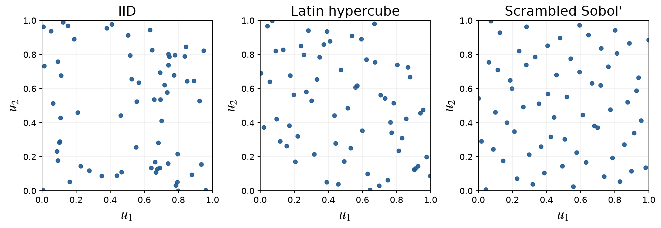
Each design has \(n=64\) points in \([0,1]^2\)
Strengths and limitations of LHS
Strengths
No importance density, control variate, or conditional expectation requiredCan converge faster than IID sampling
Guarantees one point in every one-dimensional stratum
Limitations
The sample size is fixed when the design is constructed
Accuracy assessment requires independent replications
Too many replications can erase the efficiency gain
The one-dimensional \(n^{-3/2}\) RMSE guarantee does not extend automatically to \(d>1\)
The van der Corput sequence
Low
Write a nonnegative integer in base \(b\) :
\[
i=(\cdots i_2i_1i_0)_b
\]
Reverse the digits across the radix point:
\[
\phi_b(i)=(0.i_0i_1i_2\cdots)_b
=\frac{i_0}b+\frac{i_1}{b^2}+\frac{i_2}{b^3}+\cdots
\]
Usually \(b\) is prime; \(b=2\) is common
\(\{\phi_b(i)\}_{i=0}^{b^m-1}\) contains the same points as \(\{i/b^m\}_{i=0}^{b^m-1}\) in a different orderEarlier points keep their order as the sample grows
The van der Corput construction turns a fixed-size grid into an extensible sequence
First points in base two
For \(i=0,1,2,3\) , reversing the binary digits gives
\[
\bigl(\phi_2(0),\phi_2(1),\phi_2(2),\phi_2(3)\bigr)
=\bigl(0,\frac12,\frac14,\frac34\bigr)
\]
The first four points form the grid \(\{0,1/4,1/2,3/4\}\) in a different order
\(\exstar\) Compute \(\phi_2(4)\) and \(\phi_2(5)\) and identify the two new eighths
\(\exstar\) Compute \(\phi_2(9)\) , \(\phi_2(14)\) , and \(\phi_2(19)\) by reversing their binary digits
The new values are \(1/8\) and \(5/8\) , respectively: reverse the three binary digits in \(4=100_2\) and \(5=101_2\) across the radix point. For the larger indices, \(9=1001_2\) , \(14=1110_2\) , and \(19=10011_2\) give \(\phi_2(9)=9/16\) , \(\phi_2(14)=7/16\) , and \(\phi_2(19)=25/32\) .
Four low discrepancy families
Low
For \(i=0,1,\ldots\) :
Kronecker
\(\vu_i=i\vzeta\bmod1\) none
Lattice
\(\vu_i=\phi_b(i)\vzeta\bmod1\) \(n=b^m\)
Halton
\(\vu_i=(\phi_2(i),\phi_3(i),\phi_5(i),\ldots)\) none
Digital
\(\vu_i=i_0\vc_0\oplus i_1\vc_1\oplus\cdots\) \(n=b^m\)
Here \(\oplus\) denotes digitwise addition modulo \(b\)
For basic Halton, choosing the coordinate bases fixes the sequence
Different families balance extensibility , projection quality , and fast construction
Low Discrepancy Constructions notebook : recover generators from the first points
Lattice sequence: eight points
For the lattice sequence with \(b=2\) , generator \(\vzeta=(1,3)\) , and \(n=8\) ,
\[
\vu_i=\phi_2(i)\vzeta\bmod1
\]
0
000
\(0\) \(0\) \(0\)
1
001
\(1/2\) \(1/2\) \(1/2\)
2
010
\(1/4\) \(1/4\) \(3/4\)
3
011
\(3/4\) \(3/4\) \(1/4\)
4
100
\(1/8\) \(1/8\) \(3/8\)
5
101
\(5/8\) \(5/8\) \(7/8\)
6
110
\(3/8\) \(3/8\) \(1/8\)
7
111
\(7/8\) \(7/8\) \(5/8\)
For example, \(i=5\) gives \(\phi_2(5)=5/8\) and \(3(5/8)=15/8\equiv7/8\pmod1\)
Kronecker sequence: four points
For hand arithmetic, take \(\vzeta=(0.41,0.73)\) and \(\vu_i=i\vzeta\bmod1\)
0
\(0\) \(0\) \((0,0)\)
1
\(0.41\) \(0.73\) \((0.41,0.73)\)
2
\(0.82\) \(1.46\bmod1=0.46\) \((0.82,0.46)\)
3
\(1.23\bmod1=0.23\) \(2.19\bmod1=0.19\) \((0.23,0.19)\)
The decimal generator keeps this finite example easy to calculate by hand
Digital sequence: four points
In base two, let \(i=i_0+2i_1\) and choose \(\vc_0=(1/2,1/2)\) , \(\vc_1=(1/4,3/4)\)
0
00
none
\((0,0)\)
1
01
\(\vc_0\) \((1/2,1/2)\)
2
10
\(\vc_1\) \((1/4,3/4)\)
3
11
\(\vc_0\oplus\vc_1\) \((3/4,1/4)\)
For \(i=3\) , add binary digits without carrying: \((0.10_2,0.10_2)\oplus(0.01_2,0.11_2)=(0.11_2,0.01_2)\)
Construct with new generators
\(\exstar\) Lattice: Keep \(b=2\) and \(n=8\) , but use \(\vzeta=(1,5)\) ; find \(\vu_4\) and \(\vu_5\) using the \(\phi_2(i)\) values in the table
\(\exstar\) Kronecker: Use \(\vzeta=(0.73,0.24)\) ; find \(\vu_2\) and \(\vu_3\) to two decimal places
\(\exstar\) Digital , \(b=2\) : Use \(\vc_0=(1/2,1/4)\) , \(\vc_1=(1/4,1/2)\) , and \(\vc_2=(1/8,3/8)\) ; find \(\vu_i\) for \(i=0,\ldots,7\)
Lattice: \(\vu_4=(1/8,5/8)\) and \(\vu_5=(5/8,1/8)\) . Kronecker: \(\vu_2=(0.46,0.48)\) and \(\vu_3=(0.19,0.72)\) . These rational decimal generators eventually repeat, unlike the irrational generators chosen for long Kronecker sequences; here they isolate the hand calculation of \(i\vzeta\bmod1\) . Digital, in order from \(i=0\) to \(7\) : \((0,0),(1/2,1/4),(1/4,1/2),(3/4,3/4),
(1/8,3/8),(5/8,1/8),(3/8,7/8),(7/8,5/8)\) . The family table does not privilege a particular discrepancy measure; construction quality depends on the function class and the chosen criterion.
Randomized low discrepancy sampling
Low
Randomization aims for
\[
\vU_{\mathrm{rand},i}\sim\Unif[0,1]^d
\]
for every \(i\) , while preserving low discrepancy jointly
Random shift : \(\vU_{\mathrm{rand},i}=\vu_i+\vDelta\bmod1\) , especially for lattices and Kronecker sequencesRandom digital shift : \(\vU_{\mathrm{rand},i}=\vu_i\oplus\vDelta\) , especially for digital sequencesLinear matrix or nested uniform scrambling , especially for digital sequences
Independent randomizations support error assessment without reverting to IID point placement; recall the earlier variance and RMSE comparison
Each randomized point is marginally uniform, so its sample mean is unbiased. Randomization almost surely avoids exact cube-boundary points, making Gaussian quantile transforms finite. The opening variance slide states the nearly \(\Order(n^{-3/2})\) RMSE rate for sufficiently smooth integrands under nested scrambling.
Shift the points you constructed
\(\exstar\) Lattice: For your \(\vzeta=(1,5)\) points, suppose the random shift is \(\vDelta=(1/4,1/2)\) ; find \((\vu_4+\vDelta)\bmod1\) and \((\vu_5+\vDelta)\bmod1\)
\(\exstar\) Digital , \(b=2\) : For your points from \(\vc_0,\vc_1,\vc_2\) , suppose the digital shift is \(\vDelta=(3/8,1/4)\) ; find \(\vu_0\oplus\vDelta\) and \(\vu_7\oplus\vDelta\)
Lattice: \(\vu_4=(1/8,5/8)\) shifts to \((3/8,1/8)\) , and \(\vu_5=(5/8,1/8)\) shifts to \((7/8,5/8)\) . Digital: \(\vu_0=(0,0)\) shifts to \((3/8,1/4)\) , and \(\vu_7=(7/8,5/8)\) shifts by binary digitwise addition to \((1/2,7/8)\) . The displayed shifts are particular realizations used for hand calculation; the random shift is uniform on the unit square in the sampling method.
Component-by-component construction
Low
Discrepancy
Generators for lattice rules and digital nets may be chosen by number theory or computer search
The component-by-component strategy:
Choose a one-dimensional generator that minimizes a discrepancy criterion over relevant sample sizes
Freeze the first \(\ell\) components
Search for component \(\ell+1\) that minimizes discrepancy
Increase \(\ell\) and repeat until \(\ell=d\)
A high-dimensional design is built by optimizing one coordinate at a time
Stopping criteria
Data-Driven
Error
Two practical questions are
\[\begin{align*}
\abs{\mu-\hmu_n}&\le\text{what?}\\
\abs{\mu-\hmu_n}&\le\varepsilon
\quad\text{for what $n$?}
\end{align*}\]
Use the computed contributions: \(Y_i\) , \(Y_{\mathrm{IS},i}\) , \(Y_{\mathrm{CV},i}\) , or \(Y_{\mathrm{CMC},i}\)
IID sampling: use a Central Limit Theorem interval when justified
Randomized low discrepancy sampling: use independent replications
Coefficient-decay bounds: Fourier for lattices, Walsh for digital nets
Further approach: Bayesian credible intervals based on a kernel model
An efficient method needs both fast error decay and a reliable stopping rule
Stopping rules in action
Read each run’s tolerance , estimate, reported interval or bound, sample count, and decision
Budget exhausted \(\ne\) tolerance met
Approximate intervals and conditional bounds need their stated assumptions
The Keister reference is checked only after stopping. The IID interval uses a pilot-sized final run; the replication interval uses independent scrambles, not the within-scramble sample variance. Nominal fixed-sample interval coverage does not automatically carry over to adaptive stopping. Walsh-decay guarantees assume cone membership, which passing necessary-condition checks cannot prove. For the Asian option, distinguish simulation error from model and discretization error, and include the pilot in the computational budget. The linked low discrepancy constructions notebook compares fixed sample sizes without duplicating these stopping demonstrations.
Read a stopping decision
Results from the Keister stopping comparison
IID CLT
\(0.005\) \(0.00472\) \(0.00117\)
Walsh bound
\(0.005\) \(0.00284\) \(0.000118\)
Sobol’, tight budget
\(10^{-7}\) \(0.00184\) \(0.00094\)
\(\exstar\) Interpret the reported uncertainty Which runs meet the reported tolerance? Why must the reference stay out of the stopping decision? What assumptions qualify the IID interval and Walsh bound?
The first two reported radii meet their requested tolerances; the tight-budget run does not. Reaching the budget is not success. The reference is an independent diagnostic available for this benchmark, not information normally available to choose the sample count for an unknown integral. One observed actual error also cannot establish coverage or a general guarantee. The IID interval is approximate, based on a CLT, estimated variance, and the independent-pilot design. The Walsh bound assumes membership in its specified function cone; passing necessary-condition checks does not prove membership. Adaptive replication intervals need the additional coverage qualification already stated in the notebook. Numbers are rounded from the saved run; random seeds, tolerances, or code changes can produce different results.