MATH 476 — Statistics
Introduction and Probability Review
Wackerly et al. Ch. 1–7 (parts)
Diagnostic Quiz due 1/16
Assignment 2 due 1/30
May 19, 2026
Slide Decks for This Course
How to read these slides
These slides are written in Quarto and the source code is available on the class repository, MATH476Spring2026 on GitHub
This is a link to somewhere else, in this case the title slide
This color means emphasis
| Abbreviation | Text or Reference |
|---|---|
CB |
G. Casella & R. L. Berger, Statistical Inference, 2nd ed. (2002) |
WMS |
D. S. Wackerly, W. Mendenhall III, & R. L. Scheaffer, Mathematical Statistics with Applications, 7th ed (2008) |
EH |
B. Efron & T. Hastie, Computer Age Statistical Inference (2016) |
Mathematical formulas are written in LaTeX syntax, e.g., \(\me^{\pi i} + 1 = 0\) or \[ \int_a^b f(x) \, \dif x \approx \sum_{i=1}^n w_i f(x_i) \]
Statistics
- Clear assumptions
- Probability as a basis
- Efficient and accurate computation
- Want to know parameters that describe a large number of individuals or the relationships among them
- Should provide a level of uncertainty
- Carefully sampled
- Observations, surveys, experiments, or computer simulations
Examples
Let’s look at
Approval ratings
The Gallup Poll tracks the approval ratings of US presidents according to a careful polling methodology
- Each week they telephone \(n=1500\) adults
- Their sampling error for the approval ratings is about \(4\%\)
Let \(Y \sim \Bern(\mu)\), a Bernoulli (free throw shooting) distribution with probability of success \(\mu\), \[ \Prob(Y =y) = \begin{cases} \mu, & y=1, \text{ (yes, approve)}\\ 1-\mu, & y = 0, \text{ (no, do not approve)} \end{cases} \]
If \(Y_1, \ldots, Y_n \IIDsim \Bern(\mu)\), then \[\begin{align*} T &:= Y_1 + \cdots + Y_n \sim \Bin(n,\mu), \; \Prob(T = t) = \binom{n}{t} \mu^t (1-\mu)^{n-t}\\ \barY &:= \frac 1n (Y_1 + \cdots + Y_n) \\ & \appxsim \Norm\bigl(\mu,\mu(1-\mu)/n\bigr) \quad \text{by the }\class{alert}{\text{Central Limit Theorem}} \end{align*}\]
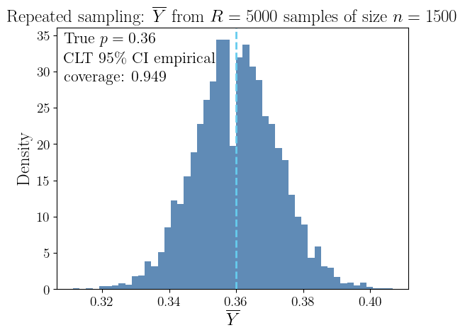
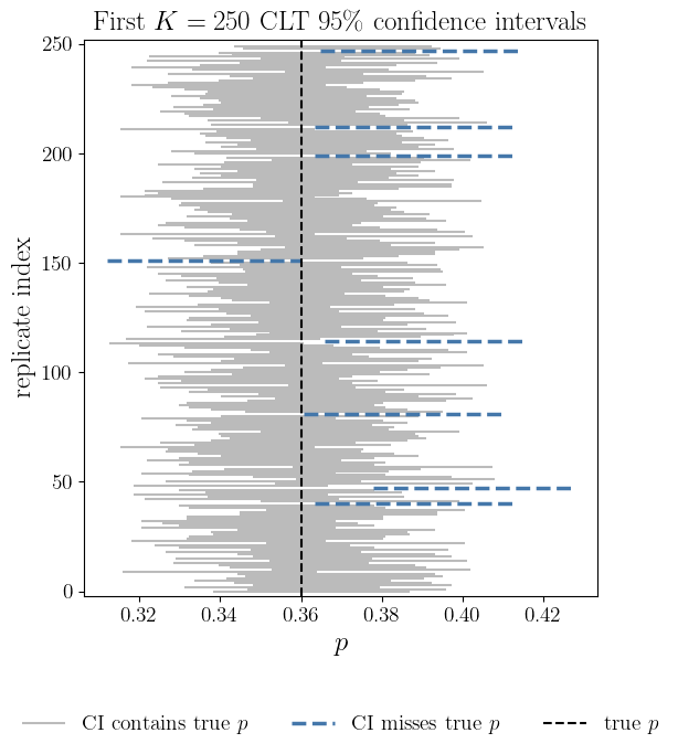
If \(Y_1, \ldots, Y_n \IIDsim \Bern(\mu)\), then we can construct a confidence interval that captures the true approval rating with high probability: \[\begin{align*} T &:= Y_1 + \cdots + Y_n \sim \Bin(n,\mu), \quad \Prob(T = t) = \binom{n}{t} \mu^t (1-\mu)^{n-t}\\ \barY &:= \frac 1n (Y_1 + \cdots + Y_n) \appxsim \Norm\bigl(\mu,\mu(1-\mu)/n\bigr) \quad \text{by the }\class{alert}{\text{Central Limit Theorem}} \end{align*}\]
\[\begin{align*} 95\% & \approx \Prob\Bigl[\mu - 1.96\sqrt{\mu(1-\mu)/n} \le \class{alert}{\barY} \le \mu + 1.96\sqrt{\mu(1-\mu)/n}\Bigr] \\ & = \Prob\Bigl[\barY - 1.96\sqrt{\mu(1-\mu)/n} \le \class{alert}{\mu} \le \barY + 1.96\sqrt{\mu(1-\mu)/n}\Bigr] \\ & \approx \Prob\Bigl[\barY - 1.96\sqrt{\barY(1-\barY)/n} \le \class{alert}{\mu} \le \barY + 1.96\sqrt{\barY(1-\barY)/n}\Bigr] \\ & \le \Prob\Bigl[\barY - 1/\sqrt{n} \le \class{alert}{\mu} \le \barY + 1/\sqrt{n} \Bigr] \quad \text{since } \sqrt{\barY(1-\barY)} \le 1/2 \end{align*}\] For \(n = 1000\) we get \(1/\sqrt{n} \approx 3\%\). ⬇ Approval Rating Jupyter 📓
- Population is US adults
- Model
- Bernoulli distribution
- Ignores demographic factors that might explain approvals
- Uncertainty of the estimate of the proportion, \(\mu\)
- Provided by a confidence interval (CI)
- Facilitated by the Central Limit Theorem
- This is the CI capturing \(\mu\), not probability of \(\mu\) in the CI
Life expectancy vs gross domestic product (GDP) per capita
Countries differ dramatically in both life expectancy and economic output. A classic dataset (World Bank / Gapminder) records, for each country,
- Life \(=\) Life expectancy at birth (years)
- GDP \(=\) Gross domestic product per capita (USD, purchasing-power adjusted)
Each point represents one country, not one individual. We are interested in the conditional behavior of life expectancy with given national income:
\[ \Ex(\text{Life} | \text{GDP} = x) \]
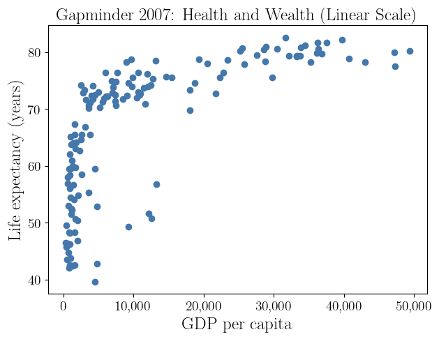
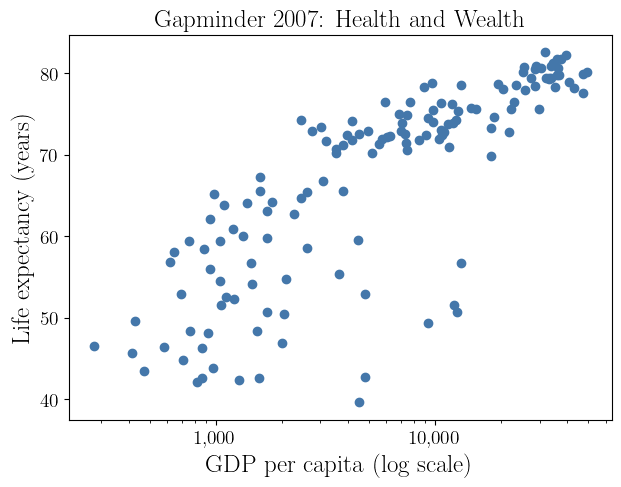
The scatterplot of life expectancy versus GDP per capita reveals two important statistical features.
Nonlinearity
Increases in GDP have a much larger effect on life expectancy at low income levels than at high income levels
Heteroscedasticity
Countries with low GDP exhibit much greater variability in life expectancy
Take logarithm to treat this \[ \Ex(\text{Life} \mid \text{GDP} = x) \approx \alpha + \beta \log(x) \]
- \(\beta\) measures years of life gained per multiplicative increase in GDP
- The log scale naturally reflects diminishing returns
- Population is all hypothetical countries
- Model
- Linear regression
- Incorporates transformation of the explanatory variable
- Uncertainty
- \(R^2\) measures the proportion of variance in \(Y\) captured by the model
- Interpretation
- This describes relationship, not cause and effect
- The variation in the residuals point to other explanatory factors that have been left out of the model
Numerical integration
Computational mathematics seems distinct from statistics, but there is an overlap.
Suppose that \(f\) is a random function defined in \([0,1]\), in particular, a Gaussian process, i.e., \(f \sim \GP(0,K)\). This means that for any distinct \(x_1, \ldots, x_n \in [0,1]\), the random vector of function values, \(\vf := \bigl(f(x_1), \ldots, f(x_n) \bigr)^\top\), has a multivariate Gaussian distribution with
- Mean \(\vmu = \Ex(\vf) = \vzero\)
- Covariance matrix \(\mSigma := \Ex(\vf \vf^\top) = \bigl(\Ex[f(x_i)f(x_j)]\bigr)_{i,j=1}^n = \bigl(K(x_i,x_j)\bigr)_{i,j=1}^n =: \mK\)
If this is the Bayesian prior belief about \(f\), then the Bayesian posterior mean of the function conditioned on the data \(\vf = \vy\) is \[ \Ex\bigl[f(x) \mid \vf = \vy\bigr] = \vy^\top \mK^{-1} \vk(x) , \quad \text{where } \vk(x) = \bigl( K(x,x_i) \bigr)_{i=1}^n \]
The Bayesian posterior mean integral of \(f\) conditioned on the data is
\[ \Ex\biggl[\int_0^1 f(x) \, \dif x \mid \vf = \vy\biggr] = \vy^\top \mK^{-1} \int_0^1 \vk(x) \, \dif x \]
For \(K(t,x) = 2 - \lvert t - x\rvert\) this is the trapezoidal rule. ⬇ Bayesian Quadrature 📓
- Population all (continuous) functions
- Model
- Stochastic processes
- Bayesian inference
- Often one would estimate the parameters in \(K\) from data
- Uncertainty
- You may construct Bayesian credible intervals, but they depend on your confidence in choosing a reasonable \(K\)
- Interpretation
- Provides a statistical interpretation of computational mathematics
Class complexion
| Familiarity | Statistics | Probability | Matrix algebra | Multivariate calculus | Computer programming / coding |
|---|---|---|---|---|---|
| Not at all | 0 | 0 | 1 | 1 | 0 |
| A bit | 4 | 3 | 1 | 4 | 1 |
| Somewhat | 10 | 5 | 8 | 7 | 10 |
| Rather | 11 | 10 | 10 | 12 | 11 |
| Very | 0 | 7 | 4 | 1 | 3 |
| Programming environments | |
|---|---|
| Python | 24 |
| R | 11 |
| MATLAB | 4 |
| C/C++ | 1 |
| Java/Javascript | 4 |
| Fortran | 1 |
Probability Review
Key probability concepts
(CB Ch. 1–2; WMS Ch. 1–2)
Outcome — a single possible result of a random process, e.g.,
yes, \(0.5\), \((1,-2)\).Sample space — the set of all possible outcomes, e.g., \(\{\text{yes},\text{no}\}\), \(\reals\).
Event — a subset of the sample space to which we may assign a probability, e.g., intervals like \([0,\infty)\) or regions such as \(\{(x,y) : x^2 + y^2 \le 1\}\).
Event space — a collection of events (subsets of the sample space) that we are allowed to assign probabilities to.
Probability — a function \(\Prob:\text{event space}\to[0,1]\) satisfying:
- \(0 \le \Prob(A) \le 1\) for every event \(A\)
- \(\Prob(\text{sample space}) = 1\)
- If \(A \cap B = \varnothing\), then \(\Prob(A \cup B) = \Prob(A) + \Prob(B)\)
Random variable/vector/function — rule that assigns a number (or vector) to each outcome, e.g., \(Y = 1\) if approve, \(0\) if not; \(X = \text{time to wait for taxi}\); \(\vX = (\text{height}, \text{weight})\)
Cumulative distribution function (CDF) \(F\) of random variable \(X\) (right-continuous)
- \(F(x) : = \Prob(X \le x)\)
- Survival function \(S(x) := \Prob(X > x) = 1 - F(x)\)
Quantile function \(Q\) of a random variable \(X\) plays the role of the inverse of the CDF (in a left-continuous sense)
- \(Q(p) : = \inf\{x \in \reals : F(x) \ge p\}, \quad 0 < p < 1\)
Probability density function (PDF) \(\varrho\) of an absolutely continuous random variable \(X\)
- \(\varrho(x) := F'(x)\)
- Expectation — average value of a random variable, weighted by its probability
- \(\displaystyle \Ex[f(X)] : = \sum_{x} f(x) \varrho(x)\) for discrete random variables
- \(\displaystyle \Ex[f(X)] : = \int f(x) \varrho(x) \, \dif x\) for continuous random variables
- \(\displaystyle \Ex[f(X)] : = \int f(x) \, \dif F(x)\) in general (see Lebesgue–Stieltjes integral)
- Mean of \(X\) is \(\mu : = \Ex(X) \exeq \Argmin{m\in\reals} \Ex[(X-m)^2]\)
- \(\Ex(a X + Y) \exeq a \Ex(X) + \Ex(Y)\)
- Variance of \(X\) is \(\sigma^2 : = \var(X) := \Ex[(X - \mu)^2] \exeq \Ex(X^2) - \mu^2\)
- Standard deviation of \(X\) is \(\std(X) := \sigma = \sqrt{\var(X)}\)
- Median of \(X\) is \(\med(X) : = Q(1/2) \in \Argmin{m\in\reals} \Ex (\lvert X-m \rvert)\)
\((X,Y)\) are independent iff \(F_{X,Y}(x,y) = F_X(x) F_Y(y)\) for all \(x,y\)
- or equivalently \(\varrho_{X,Y}(x,y) = \varrho_X(x) \varrho_Y(y)\) for all \(x,y\)
Covariance \(\cov(X,Y) : = \Ex[(X- \mu_X)(Y - \mu_Y)]\)
- \(\var(aX + Y) \exeq a^2 \var(X) + \var(Y)\) if \(\cov(X,Y) = 0\)
Correlation \(\displaystyle \corr(X,Y) : = \frac{\cov(X,Y)}{\std(X) \std(Y)}\)
Independence \(\implies\) zero correlation, but zero correlation \(\notimplies\) independence
- E.g., \(\Prob[(X,Y) = (x,y)] = 1/4\) for \((x,y) \in \{(\pm 1, 0), (0, \pm 1)\}\) \[\begin{gather*} \text{PMF }\varrho_X(x) = \varrho_Y(x) = \begin{cases} \frac 14 & x = \pm 1 \\ \frac 12 & x = 0 \end{cases} \qquad \Ex(X) = \Ex(Y) = 0 \\ \cov(X,Y) = \Ex(XY) = 0 \quad \text{so }\class{alert}{\text{uncorrelated}} \\ \text{BUT } \varrho_{XY}(x,y) \ne \varrho_X(x)\varrho_Y(y) \quad \text{so }\class{alert}{\text{dependent}} \end{gather*}\]
Important distributions
(CB §§3.1–3.3; WMS §§3.1–3.4, §§4.1–4.6)
Binomial (free-throw shooting, discrete) \(\Bin(n,p)\) \[ \varrho(x) : = \Prob(X=x) = \binom{n}{x} p^x (1-p)^{n-x}, \ x =0, \ldots, n; \quad \Ex(X) = np, \; \var(X) = np(1-p) \]
Exponential (taxi waiting, continuous) \(\Exp(\lambda)\) \[ F(x): = 1 - \exp(-\lambda x),\ \varrho(x) : = \lambda \exp(-\lambda x), \ x \ge 0; \quad \Ex(X) = 1/\lambda, \quad \var(X) = 1/\lambda^2 \]
Uniform (random number generation, continuous) \(\Unif(a,b)\) \[\begin{gather*} F(x) : = \begin{cases} 0, & -\infty < x < a, \\ \displaystyle \frac{x - a}{b - a}, & a \le x < b, \\ 1, & b \le x < \infty, \end{cases} \qquad \qquad \varrho(x): = \frac{1}{b-a}, \ x \in [a,b]; \\ \Ex(X) = \frac{a+b}{2}, \quad \var(X) = \frac{(b-a)^2}{12} \end{gather*}\]
Normal (Gaussian) (limiting distribution, continuous) \(\Norm(\mu, \sigma^2)\) \[ \varrho(x): = \frac{\exp\bigl(-(x-\mu)^2/(2\sigma^2)\bigr)}{\sqrt{2 \pi} \sigma}, \ x \in \reals;\quad \Ex(X) = \mu, \quad \var(X) = \sigma^2 \]
Multivariate Normal (Gaussian) (limiting distribution, continuous) \(\Norm(\vmu, \mSigma)\) \[\begin{gather*} \varrho(\vx): = \frac{\exp\bigl(-(\vx-\vmu)^\top \mSigma^{-1} (\vx-\vmu) /2\bigr)}{\sqrt{(2 \pi)^{d} \det(\mSigma)}};\; \Ex(\vX) = \vmu, \\ \cov(\vX) = \mSigma \class{alert}{\text{ symmetric, positive definite covariance matrix}} \end{gather*}\]
A mixed (partially discrete, partially continuous) random variable
- Discrete random variables have a PMF
- Continuous random variables have a PDF
- Some random variables are mixed
Zero-inflated exponential distribution — \(X\) is the waiting time for a taxi
- A taxi waiting for you with probability \(p\)
- But if there is none, then the waiting time is exponential with mean \(1/\lambda\) \[\begin{align*} F(x) &= \begin{cases} 0, &-\infty < x < 0 \\ 1- (1-p)\exp(-\lambda x), & 0 \le x < \infty \end{cases} \end{align*}\] Note: \(F\) has a jump of size \(p\) at \(x=0\), corresponding to \(\Prob(X=0)=p\)
\[\begin{align*} \mu & = \Ex(X) = \int_{-\infty}^{\infty} x \, \dif F(x) \qquad \mathlink{https://en.wikipedia.org/wiki/Lebesgue-Stieltjes_integration}{(Lebesgue–Stieltjes integral)}\\ & = \underbrace{0 \times p}_{\text{from the jump at } 0} + \int_0^{\infty} x \times (1-p) \lambda \exp(-\lambda x) \, \dif x = (1-p)/ \lambda \\ \sigma^2 & = \var(X) = \Ex(X^2) - \mu^2 \exeq \frac{1-p^2}{\lambda^2} \end{align*}\]
Lebesgue–Stieltjes integral = integral + jumps
Let the CDF \(F\)
- Be a nondecreasing, right-continuous function on \(\mathbb{R}\)
- Have (possible) discontinuities at \(-\infty < x_1 < \ldots < x_N < \infty\)
- Be differentiable between its jump points, with \(\varrho(x)=F'(x)\) there
and let \(f\) be a suitable function
The Lebesgue–Stieltjes integral of \(f\) with respect to \(F\) can be written as \[\begin{align*} \int f(x)\, dF(x) & = \int_{-\infty}^{x_{1}} f(x) \,\varrho(x) \, \dif x + \sum_{k=1}^{N-1} \int_{x_k}^{x_{k+1}} f(x) \, \varrho(x) \, \dif x + \int_{x_N}^{\infty} f(x) \, \varrho(x) \, \dif x \\ & \qquad \qquad + \sum_{k=1}^N f(x_k)[F(x_k) - F(x_k^{-})] \end{align*}\]
Integrate \(f\) where \(F\) is smooth, and add a weighted sum of \(f\) at the jump points of \(F\)
Conditional probability
(CB §1.3, §4.2; WMS 2.7)
The conditional probability means restricting attention to outcomes where \(B\) occurs, then measure how often \(A\) occurs within that restricted universe of \(A\) given \(B\) (with \(\Prob(B)>0\)): \[ \Prob(A \mid B) = \frac{\Prob(A \cap B)}{\Prob(B)}, \] which means restricting attention to outcomes where \(B\) occurs, then measuring how often \(A\) occurs within that restricted universe.
Multiplication rule: \(\Prob(A \cap B) = \Prob(A \mid B) \Prob(B)\)
\(A\) and \(B\) are independent if \(\Prob(A \mid B) = \Prob(A)\) or equivalently \(\Prob(A \cap B)=\Prob(A)\Prob(B)\)
Bayes’ Rule
\[ \Prob(A \mid B) = \frac{\Prob(B \mid A) \, \Prob(A)}{\Prob(B)}, \qquad \Prob(B)>0 \]
Let \(X\) and \(Y\) have joint density \(\varrho_{X,Y}(x,y)\). The conditional density of \(X\) given \(Y=y\) is \[ \varrho_{X\mid Y}(x \mid y) = \frac{\varrho_{X,Y}(x,y)}{\varrho_Y(y)}, \qquad \varrho_Y(y)=\int \varrho_{X,Y}(x,y) \, \dif x \text{ is the }\class{alert}{\text{marginal density}} \text{ of } Y \]
Bayes’ rule for densities
\[ \varrho_{X\mid Y}(x\mid y) = \frac{\varrho_{Y\mid X}(y\mid x)\,\varrho_X(x)}{\varrho_Y(y)} \]
\(\exstar\) If you meet an introvert, is she more likely to be a librarian or a salesman?
\(\exstar\) What probability distributions defined on \([0,\infty)\) satisfy the memoryless property, i.e. \(\Prob[X > t + x | X > t] = \Prob[X > x]\)?
Bayesian statistics to approximate and integrate functions
We assume that \(f\), the function to approximate or integrate, is an instance of a Gaussian process, \(\GP(0,K)\). This means that
\[\begin{gather*}
\vf := \bigl(f(x_1), \ldots, f(x_n) \bigr)^\top \sim \Norm(\vzero, \mK), \quad \text{where }\mK : = \bigl(K(x_i,x_j)\bigr)_{i,j=1}^n \\
\tvf := \bigl(f(x_1), \ldots, f(x_n), f(x) \bigr)^\top \sim \Norm(\vzero, \tmK) \\
\text{where }
\tmK : = \left(\begin{array}{c|c}
\mK & \vk(x) \\
\hline
\vk^\top(x) & K(x,x)
\end{array}
\right)
, \quad \vk(x) = \bigl( K(x,x_i) \bigr)_{i=1}^n
\end{gather*}\] and so the conditional density of \(f(x)\) given \(\vf = \vy\), where \(\vy\) is the observed data, is
\[\begin{align*}
\varrho_{f(x) | \vf}(z | \vy) = \frac{\varrho_{\tvf}(\tvy)}{\varrho_{\vf}(\vy)} = \frac{\frac{\exp(-\tvy^\top \tmK^{-1} \tvy/2)}{\sqrt{(2 \pi)^{n+1} \det(\tmK)}}}{\frac{\exp(-\vy^\top \mK^{-1} \vy/2)}{\sqrt{(2 \pi)^{n} \det(\mK)}}}
= \frac{\exp([-\tvy^\top \tmK^{-1} \tvy + \vy^\top \mK^{-1} \vy]/2)}{\sqrt{(2 \pi) \det(\tmK)/\det(\mK)}}
\end{align*}\] where \(\tvy = (\vy^\top, z)^\top\)
One can show that the inverse of the covariance matrix is
\[\begin{gather*} \tmK^{-1} = \left(\begin{array}{c|c} \mK^{-1}+\mK^{-1}\vk(x)\sigma^{-2}(x)\vk^\top(x)\mK^{-1} & -\mK^{-1}\vk(x)\sigma^{-2}(x) \\ \hline - \sigma^{-2}(x)\vk^\top(x)\mK^{-1} & \sigma^{-2}(x) \end{array} \right)\\ \text{where } \sigma^2(x)=K(x,x)-\vk^\top(x)\mK^{-1}\vk(x), \qquad \sigma^{-2}(x) := \big(\sigma^2(x)\big)^{-1} \end{gather*}\]
So
\[\begin{align*} \MoveEqLeft{-\tvy^\top \tmK^{-1} \tvy + \vy^\top \mK^{-1} \vy}\\ & = -\vy^\top[\mK^{-1}+\mK^{-1}\vk(x)\sigma^{-2}(x)\vk^\top(x)\mK^{-1}]\vy + 2 \vy^\top\mK^{-1}\vk(x)\sigma^{-2}(x) z - z^2 \sigma^{-2}(x) \\ & \qquad \qquad + \vy^\top \mK^{-1} \vy \\ & = \sigma^{-2}(x) [ z - \vy^\top \mK^{-1} \vk(x)]^2 \end{align*}\]
and \(f(x) \mid \vf = \vy \sim \Norm\bigl(\vy^\top \mK^{-1} \vk(x), \sigma^2(x) \bigr)\)
By a similar argument \(\int_0 ^1 f(x)\, \dif x \mid \vf = \vy \sim \Norm\Bigl(\vy^\top \mK^{-1} \int_0^1 \vk(x) \, \dif x, \int_0^1 \int_0^1 K(t,x) \, \dif t \dif x - \int_0^1 \vk^\top(x) \, \dif x \, \mK^{-1} \, \int_0^1 \vk(x) \, \dif x \Bigr)\)
Bayesian inference
(CB §7.2.3)
\[\begin{align*} \text{Recall that}&& \varrho_{X\mid Y}(x\mid y) &= \frac{\varrho_{Y\mid X}(y\mid x)\,\varrho_X(x)}{\varrho_Y(y)} \\ \text{Let} && X & = \text{random unknown parameter} \\ && Y & = \text{random observed data} \\ && \varrho_X & = \text{prior density or belief about the parameter} \\ &&\varrho_{Y\mid X} & = \text{likelihood} \\ && \varrho_{X\mid Y} & = \text{posterior density} \\ \text{Then} && \varrho_{X\mid Y}( \text{parameter} \mid \text{data}) & = \frac{\varrho_{Y\mid X}(\text{data}\mid \text{parameter} ) \,\varrho_X(\text{parameter})}{\varrho_Y(\text{data})} \\ && \text{posterior density } & \propto \text{likelihood} \times \text{prior density} \end{align*}\]
Conditional expectation
Conditional expectation of \(X\) given event \(A\) (with \(\Prob(A)>0\)) is \[ \Ex[X \mid A] = \frac{\Ex[X \, \indic(X \in A)]}{\Prob(A)} \qquad \text{and so} \qquad \Ex[X \, \indic(X \in A)] = \Prob(A)\,\Ex[X \mid A] \] The indicator function, \(\indic(\cdot)\), equals \(1\) if the statement inside the parentheses is true, and \(0\) otherwise.
Conditional expectation of \(X\) given \(Y=y\) is \[ \Ex[X \mid Y=y] = \int x \, \varrho_{X\mid Y}(x \mid y)\,\dif x \] If \(g(y)=\Ex[X \mid Y=y]\), then \(\Ex[X \mid Y] = g(Y)\) is a random variable depending only on \(Y\)
If \(X\) is independent of \(Y\), then \(\Ex[X \mid Y] = \Ex[X]\)
Conditioning on an event
For any event \(A\) with \(0<\Prob(A)<1\), \[ \Ex[X] = \Prob(A)\,\Ex[X \mid A] + \Prob(A^c)\,\Ex[X \mid A^c] \]
More generally, if \(\{A_1,\ldots,A_n\}\) is a partition of the sample space with \(\Prob(A_i)>0\), then \[ \Ex[X] = \sum_{i=1}^n \Prob(A_i)\,\Ex[X \mid A_i]. \]
Law of total expectation
\[ \Ex\!\bigl[\Ex[X \mid Y]\bigr] = \Ex[X] \]
Law of total variance
\[ \var(X) = \Ex\!\bigl[\var(X \mid Y)\bigr] + \var\!\bigl(\Ex[X \mid Y]\bigr) \]
Types of convergence
(CB §§5.5) Let \(X_1, X_2, \ldots\) be random variables and \(X\) another random variable
Almost Sure Convergence
\[ X_n \convas X \iff \Prob \left( \lim_{n \to \infty} X_n = X \right) = 1 \] For almost every outcome the sequence \(X_n\) converges to \(X\)
Convergence in Probability
\[ X_n \convp X \iff \forall \varepsilon > 0, \; \Prob\big( |X_n - X| > \varepsilon \big) \;\longrightarrow\; 0. \] The probability that \(X_n\) differs significantly from \(X\) goes to zero
Convergence in Distribution
\[ X_n \convd X \iff \lim_{n \to \infty} F_{X_n}(x) = F_X(x) \quad \text{for all continuity points of } F_X \] The distributions of \(X_n\) approach the distribution of \(X\)
Convergence strength
\[ X_n \convas X \;\Longrightarrow\; X_n \convp X \;\Longrightarrow\; X_n \convd X, \] and none of the reverse implications hold in general
\(X, X_1, X_2, \ldots \IIDsim \Norm(0,1)\) satisfies \(X_n \convd X\), but \(X_n \nconvp X\)
\(X=0\) and \(\Prob(X_n =x ) = \begin{cases} 1/n, & x=1 \\ 1-1/n, & x=0 \end{cases} \;\) satisfies \[ \Prob(\lvert X_n - X \rvert > \varepsilon ) = \Prob(X_n =1) = 1/n \to 0 \text{ as } n \to \infty \text{ so } X_n \convp X \] Assuming the \(X_n\) are independent, \(\Prob (X_n =1 \text{ infinitely often}) = 1\) since \[ \sum_{n=1}^{\infty} \Prob(X_n=1) = \sum_{n=1}^{\infty} \frac 1n = \infty \] so \(X_n \ \, \nconvas X\)
Central Limit Theorem
(CB §5.5; WMS §§7.3–7.5)
If \(X_1, X_2, \ldots \IIDsim\) some distribution with finite moment generating function, \(M(t) := \Ex\bigl(\exp(tX_1)\bigr)\), that exists for \(t\) near \(0\), and \(\mu = \Ex(X_1)\) and \(\sigma^2 = \var(X_1)\), and \[ \barX_n := \frac 1n \left(X_1 + \cdots + X_n \right), \] then \[ \frac{\barX_n - \mu}{\sigma /\sqrt{n}} \convd \Norm(0,1) \] Note that IID means independent and identically distributed
Proof of the Central Limit Theorem
- Define a standardized (mean \(0\), variance \(1\)) random variable, \(Y_i := (X_i - \mu)/\sigma\) and note that \(Y_1, Y_2, \dots\) are IID with mean \(0\) and variance \(1\):
\[\begin{align*} Z_n: &= \frac{\barX_n - \mu}{\sigma /\sqrt{n}} = \frac{Y_1 + \cdots + Y_n}{\sqrt{n}} \\ M_{Z_n}(t) &= \Ex[\exp(tZ_n)] = \Ex[\exp(tY_1/\sqrt{n} + \cdots + tY_n/\sqrt{n})]\\ & = \Ex[\exp(tY_1/\sqrt{n}) \cdots \exp(tY_n/\sqrt{n})] \\ & = \{\Ex[\exp(tY_1/\sqrt{n})]\}^n \qquad \text{by independence} \\ & = [M_Y(t/\sqrt{n})]^n \\ \lim_{n \to \infty}M_{Z_n}(t) &= [M_Y(0)]^\infty = 1^\infty \quad \class{alert}{\text{(undetermined)}} \end{align*}\]
- Take the limit of \(M_{Z_n}(t)\) as \(n \to \infty\) using L’Hôpital’s rule \[\begin{align*} \text{Note that } M_Y(0) & = 1 \\ M'_Y(0) & = \Ex(Y_1) = 0 \\ M''_Y(0) & = \Ex(Y_1^2) = 1 \\ \text{Then }\lim_{n \to \infty} \log\bigl(M_{Z_n}(t) \bigr) & = \lim_{n \to \infty} n \log \bigl(M_Y(t/\sqrt{n}) \bigr) = \lim_{n \to \infty} \frac{\log \bigl(M_Y(t/\sqrt{n}) \bigr) }{n^{-1}} = \frac{0}{0} \quad \class{alert}{\text{(undetermined)}}\\ & = \lim_{n \to \infty} \frac{ \dfrac{-t}{2n^{3/2}} \dfrac{M'_Y(t/\sqrt{n})}{M_Y(t/\sqrt{n})} } { -n^{-2} } = \frac t2 \lim_{n \to \infty} \frac{\dfrac{M'_Y(t/\sqrt{n})}{M_Y(t/\sqrt{n})}}{ n^{-1/2} } = \frac{0}{0} \quad \class{alert}{\text{(undetermined)}} \\ & = \frac t2 \lim_{n \to \infty} \frac{ \dfrac{-t}{2 n^{3/2}} \dfrac{M_Y(t/\sqrt{n}) M''_Y(t/\sqrt{n}) - [M'_Y(t/\sqrt{n})]^2 }{ [M_Y(t/\sqrt{n})]^2}} { -n^{-3/2}/2 } = \frac{t^2}{2} \\ \lim_{n \to \infty} M_{Z_n}(t) & = \exp(t^2/2) \end{align*}\]
- Note that if \(Z \sim \Norm(0,1)\) then \[\begin{align*} M_Z(t) & = \Ex[\exp(tZ)] = \int_{-\infty}^{\infty} \frac 1{\sqrt{2 \pi}} \exp(tz - z^2/2) \, \dif z \\ & = \int_{-\infty}^{\infty} \frac 1{\sqrt{2 \pi}} \exp\bigl(-(z - t)^2/2 \bigr) \, \exp(t^2/2) \, \dif z = \exp(t^2/2) \\ &= \lim_{n \to \infty} M_{Z_n}(t) \end{align*}\]
By uniqueness of moment generating functions, \[ Z_n \convd \Norm(0,1) \] \(\square\)
Chebyshev (Markov) Inequality
(CB §3.6, §3.8) \[ \Prob\bigl( f(X) \ge r \bigr) \le \frac{\Ex[f(X)]}{r} \qquad \text{for } f \class{alert}{\text{ non-negative}}, \ r > 0 \]
Proof
\[\begin{align*} \Prob(f(X)\ge r) &= \Ex\bigl[\indic\bigl(f(X)\ge r\bigr)\bigr] \\ &= \Ex\Bigl[\Ex\bigl[\indic\bigl(f(X)\ge r\bigr)\mid X\bigr]\Bigr] \qquad \text{(total expectation)} \\ &\le \Ex\Bigl[\Ex\bigl[f(X)/r \mid X\bigr]\Bigr] \qquad \text{since } \indic\bigl(f(X)\ge r\bigr)\le f(X)/r \text{ a.s.} \\ &= \Ex\bigl[f(X)/r\bigr] = \Ex[f(X)]/r \end{align*}\]
Important special cases
\[\begin{gather*} \Prob\bigl( \lvert X - \mu \rvert^2 \ge r^2 \bigr) \le \frac{\sigma^2}{r^2} \quad \text{where } \mu = \Ex(X), \ \sigma^2 = \var(X) \\ \Prob\bigl( \lvert X - \med(X) \rvert \ge r \bigr) \le \frac{\Ex (\lvert X - \med(X)\rvert)}{r} \end{gather*}\]
Normal tails vs Chebyshev bounds
Let \(X\sim \Norm(0,1)\) and compare \(\Prob(|X|>r)\) with two bounds
Here \(\Ex\lvert X \rvert \exeq \sqrt{2/\pi} \approx 0.798\) and \(\Ex(X^2)=1\)
| \(r\) | \(\Prob(|X|>r)\) (exact) | \(\le \sqrt{2/\pi}\,/r\) (Markov) | \(\le 1/r^2\) (Chebyshev) |
|---|---|---|---|
| 1 | 0.317311 | 0.797885 (2.5×) | 1 (3.2×) |
| 2 | 0.0455003 | 0.398942 (8.8×) | 0.25 (5.5×) |
| 6 | 1.97318e-09 | 0.132981 (6.7e+07×) | 0.0277778 (1.4e+07×) |
| 10 | 1.52397e-23 | 0.0797885 (5.2e+21×) | 0.01 (6.6e+20×) |
| 100 | 0 | 0.00797885 (∞) | 0.0001 (∞) |
- The Markov and Chebyshev bounds are much looser, but more general
- CLT bounds for means will resemble the exact; we are willing to live with approximate bounds that are tighter than absolute bounds
- These guaranteed Markov and Chebyshev bounds still depend on knowing or approximating \(\sigma^2\) or \(\Ex \lvert X - \med(X)\rvert\)
Student \(t\) tails vs Markov/Chebyshev bounds
Let \(T_\nu \sim t_\nu\) and compare \(\Prob(|T_\nu|>r)\) with two bounds
| \(\nu\) | \(r\) | \(\Prob(|T_\nu|>r)\) (exact) | \(\le \Ex(|T_\nu|)/r\) (Markov) | \(\le \Ex(T_\nu^2)/r^2\) (Chebyshev) |
|---|---|---|---|---|
| 2 | 1 | 0.423 | 1.41 (3×) | inf (∞) |
| 2 | 2 | 0.184 | 0.707 (4×) | inf (∞) |
| 2 | 6 | 0.0267 | 0.236 (9×) | inf (∞) |
| 3 | 1 | 0.391 | 1.1 (3×) | 3 (8×) |
| 3 | 2 | 0.139 | 0.551 (4×) | 0.75 (5×) |
| 3 | 6 | 0.00927 | 0.184 (20×) | 0.0833 (9×) |
| 5 | 1 | 0.363 | 0.949 (3×) | 1.67 (5×) |
| 5 | 2 | 0.102 | 0.475 (5×) | 0.417 (4×) |
| 5 | 6 | 0.00185 | 0.158 (86×) | 0.0463 (25×) |
Weak Law of Large Numbers (via Chebyshev)
Theorem (WLLN)
Let \(X_1,X_2,\dots\) be IID with \(\Ex[X_1]=\mu\) and \(\var(X_1)=\sigma^2<\infty\). Define the sample mean as \(\displaystyle\barX_n := \frac1n\sum_{i=1}^n X_i\). Then \(\barX_n \convp \mu\).
Proof
By Chebyshev’s inequality, \(\displaystyle \Prob\bigl(|\barX_n-\mu|\ge \varepsilon\bigr) \le \frac{\var(\barX_n)}{\varepsilon^2}\)
Using independence, \[ \var(\barX_n) = \var\!\left(\frac1n\sum_{i=1}^n X_i\right) = \frac{1}{n^2}\sum_{i=1}^n \var(X_i) = \frac{1}{n^2}\cdot n\sigma^2 = \frac{\sigma^2}{n} \] Therefore, \[ \Prob\bigl(|\barX_n-\mu|\ge \varepsilon\bigr) \le \frac{\sigma^2}{n\varepsilon^2} \to 0 \quad \text{as } n \to \infty \qquad \square \]
Slutsky’s Theorem
If \[\begin{align*} X_n &\convd X \quad \text{and} \\ Y_n &\convp c \quad \text{for some constant } c \end{align*}\] Then \[\begin{align*} X_n + Y_n &\convd X + c \\ X_n Y_n &\convd cX \\ \frac{X_n}{Y_n} &\convd \frac{X}{c} \quad \text{if } c \neq 0 \end{align*}\]
Random quantities converging to constants behave like constants asymptotically
© 2026 Fred J. Hickernell · Illinois Tech · assisted by ChatGPT · Intro & Prob. Review · MATH 476 — Statistics Website · \(\exstar\) = exercise