MATH 476 — Statistics
Hypothesis Testing
Wackerly et al. Ch. 10
Assignment 4 due 3/13
Assignment 5 due 4/10
Fred J. Hickernell
May 19, 2026
Hypothesis Testing Framework
(CB §8.1–8.3; WMS §10.1–10.2)
Null hypothesis \(H_0\) — the default assumption, often of the form \(H_0: \theta = \theta_0\) or \(H_0: \theta \in \ct_0\)
- innocence, “no effect” or “status quo”
Alternative hypothesis \(H_A\) — the alternative, often of the form \(H_A: \theta = \theta_1\) or \(H_A: \theta \in \ct_A\)
- guilt, “effect”, or “change”
Test statistic \(T(\vX) = T_n(\vX) \in \ct\) — a function/summary of the data, \(\vX = (X_1, \ldots, X_n)\), used to assess \(H_0\)
Rejection region \(\RR \subseteq \ct\) — values of \(T(\vX)\) for which we reject \(H_0\)
Decision rule — reject \(H_0\) if \(T(\vX) \in \RR\)
Type I error \(\alpha\) — reasonable doubt, probability of falsely rejecting \(H_0\)
- \(H_0\) gets protection via the bound on Type I error
\(p\)-value — (under \(H_0\)) probability that the test statistic is at least as extreme as the observed value
Type II error \(\beta\) — probability of failing to reject \(H_0\) when \(H_A\) is true
Power \(1-\beta\) — probability of correctly rejecting \(H_0\)
Hypothesis testing is a formal way of deciding whether the data provide enough evidence to overturn a protected default assumption
We will use ideas from estimation, confidence intervals, and pivots
Example: Server Reliability Claim (Mean Time Between Failures)
Suppose
\[ X_1,\dots,X_n \IIDsim \Exp(1/\mu), \qquad \Ex(X)=\mu \]
Here
\(X_i\) is the time between unexpected server failures (e.g., crashes/outages) for a particular service
The provider claims the mean time between failures is \(\mu_0 = 200\) hours
We want evidence that reliability has worsened, i.e. failures are happening more frequently
Step 1: Hypotheses
- Null hypothesis (innocence, status quo): \(\qquad H_0:\ \mu=200\)
- Alternative hypothesis (guilty, change): \(\qquad H_A:\ \mu<200\)
Step 2: Construct test statistic
\[\text{Use the pivot } \frac{2n\barX_n}{\mu} \sim \chi^2_{2n}, \qquad \text{so that under } H_0: \mu = 200, \quad T(\vX) = \frac{2n\barX_n}{200} \sim \chi^2_{2n}\]
Step 3: Choose significance level and construct rejection region
Choose \(\alpha = 0.05\) as the maximum tolerable risk of falsely accusing underperformance
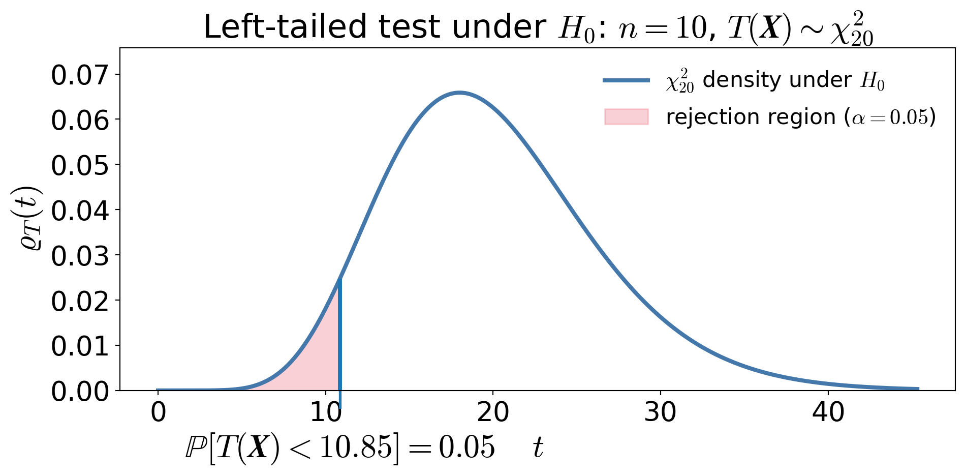
Left-tailed test:
\[\RR = [0, \chi^2_{2n,1-\alpha}) = [0, 10.85)\]
Equivalently, reject when
\[\barX_n < \frac{200}{2n}\,\chi^2_{2n,1-\alpha}\]
No data has been observed yet
Step 4: Observed Data
Let
\[n=10,\qquad \barx_n=176\]
Then \[t_{\text{obs}}=\frac{2(10)(176)}{200}=17.60\]
Step 5: \(p\)-value and decision
The \(p\)-value is
\[p=\Prob\big(\chi^2_{20} \le 17.60\big) \approx 0.39\]
Reject \(H_0\) iff \(p\le \alpha\)So we do NOT reject \(H_0\) at the \(\alpha=0.05\) level. This is not the same as accepting \(H_0\)!
Type I and Type II Errors
Type I error \(\alpha\):
Falsely conclude that reliability has worsened when the true mean time between failures is 200 hours \[\alpha=\Prob(\text{reject }H_0\mid \mu=200)\]
Type II error \(\beta(\mu_1)\) (for some \(\mu_1<200\)):
Fail to detect that the system is less reliable than claimed \[ \beta(\mu_1) = \Prob(\text{fail to reject }H_0 \mid \mu = \mu_1) \]
Power function \(\power(\mu_1)\)
The probability of correctly detecting reduced reliability (for some \(\mu_1<200\))
\[ \power(\mu_1) = \Prob(\text{reject }H_0 | \mu = \mu_1) = 1-\beta(\mu_1) \]
Power for the Server Reliability test
From Step 3, we reject \(H_0\) when
\[T(\boldsymbol{X})=\frac{2n\barX_n}{200} < \chi^2_{2n,1-\alpha}\]
If the true mean is actually \(\mu_1\), then \[\frac{200 T(\boldsymbol{X}) }{\mu_1} = \frac{2n\barX_n }{\mu_1} \sim\chi^2_{2n}\]
, the power function is \[\begin{align*} \power(\mu_1) &= \Prob\!\left(T(\boldsymbol{{X}}) < \chi^2_{2n,\,1-\alpha}\mid \mu=\mu_1\right) = \Prob\!\left(\frac{200\,T(\boldsymbol{X})}{\mu_1} \sim \chi^2_{2n} < \frac{200\,\chi^2_{2n,\,1-\alpha}}{\mu_1} \,\middle|\, \mu=\mu_1\right)\\ &\qquad \qquad \text{increases as $\mu_1$ decreases.} \end{align*}\]
Power Curves
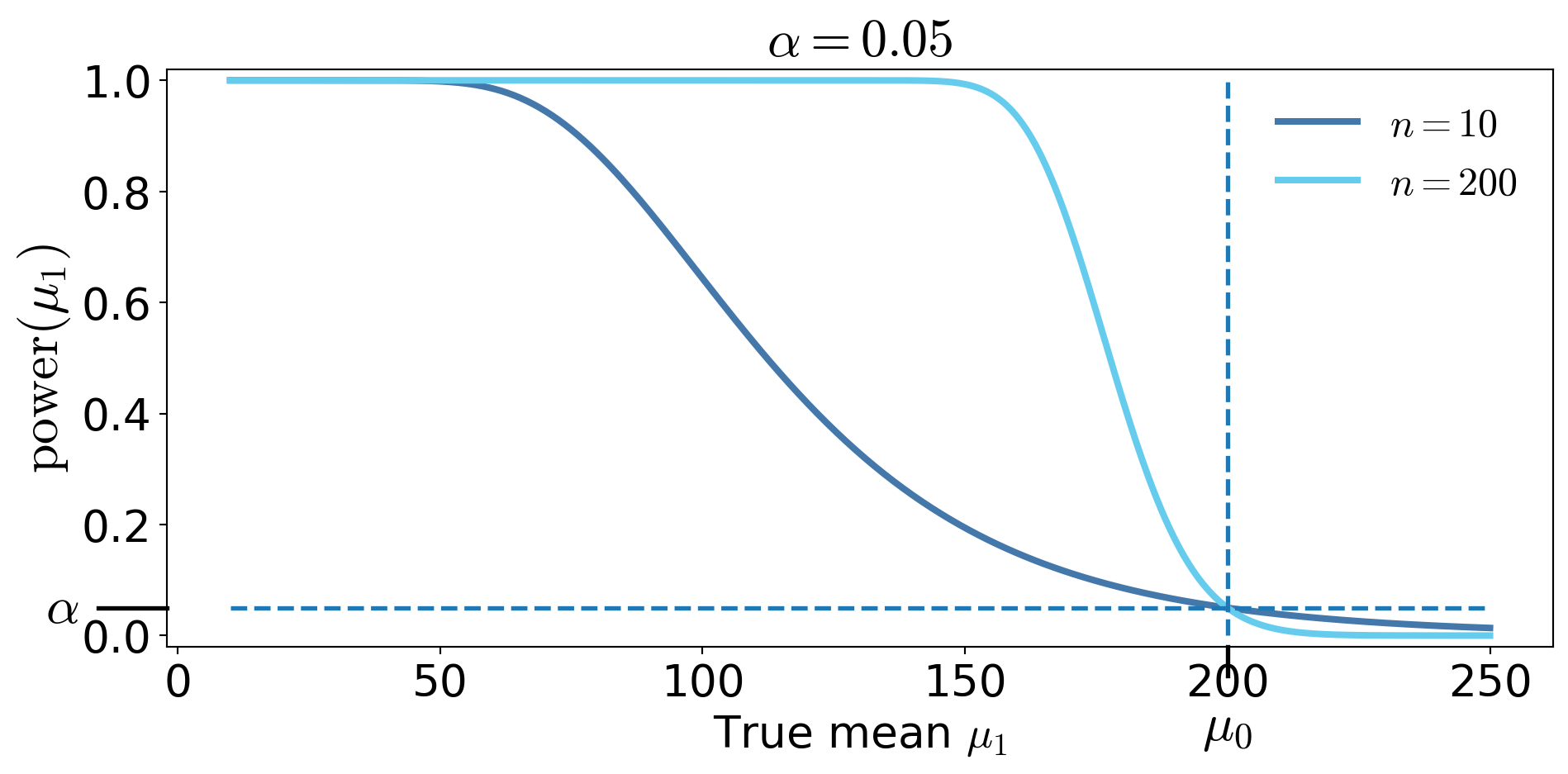
Do not use the power curve to decide whether to reject after seeing the data
Power is about the test procedure, not about the observed data
Two kinds of error
\[\begin{gather*} H_0 \text{ null hypothesis (default, innocence) in terms of } \theta \\ H_A \text{ alternative hypothesis (evidence, guilt) in terms of } \theta \end{gather*}\]
\(H_0\) and \(H_A\) are mutually exclusive
Truth vs Decision
| Reject \(H_0\) | Do Not Reject \(H_0\) | |
|---|---|---|
| \(H_0\) true | Type I error probability \(\alpha\) |
Correct |
| \(H_0\) false | Correct probability \(\power(\theta)\) |
Type II error probability \(\beta(\theta)\) |
Confidence intervals & hypothesis testing
Structural comparison
| Confidence Interval | Hypothesis Test |
|---|---|
| An interval of plausible values | A reject / do not reject decision |
| Random interval | Random decision |
| Statement about \(\theta\) | Statement about \(H_0\) |
| No special value privileged | Tests a specific value \(\theta_0\) |
Shared ingredients
| Both Use | Meaning |
|---|---|
| Level \(\alpha\) | Willingness to be wrong |
| Pivot / test statistic | Standardized measure of evidence |
| Sampling distribution | Controls coverage / Type I error |
\[ \theta_0 \text{ rejected at level } \alpha \iff \theta_0 \notin \text{corresponding } (1-\alpha) \text{ confidence interval} \]
Hypothesis Testing: Design vs Data
%%{init: {"themeVariables":{"fontSize":"36px"}}}%%
flowchart LR
  D1T["Design Phase<br/>(Before Data)"]
  D2T["Data Phase<br/>(After Data)"]

  subgraph D1 [ ]
    A[Model<br/>Assumptions]
    B[Choose Test<br/>Statistic]
    C[Sampling<br/>Distribution<br/>under null]
    D["Fix Rejection<br/>Region<br/>(size α)"]
  end

  subgraph D2 [ ]
    E[Observe<br/>Data]
    F[Compute<br/>Test<br/>Statistic]
    G[Decision:<br/>Reject or Not]
  end

  D1T --> A
  D2T --> E
  A --> B --> C --> D --> E --> F --> G

  style D1 fill:transparent,stroke:#888,stroke-width:2px
  style D2 fill:transparent,stroke:#888,stroke-width:2px

  style D1T fill:transparent,stroke:transparent,font-weight:bold
  style D2T fill:transparent,stroke:transparent,font-weight:bold
Emphasis
Everything in the Design Phase defines the procedure
- \(\alpha\) and power belong to the Design Phase
The Data Phase only applies the pre-defined rule
The power curve describes the procedure, not the observed dataset
What depends on data and what does not?
Chosen before seeing data
| Quantity | Who chooses it? |
|---|---|
| \(H_0\) and \(H_A\) | Us |
| Form of test statistic \(T\) | Us |
| Significance level \(\alpha\) | Us |
| Sample size \(n\) | Us |
| Rejection region \(\RR\) | Determined by \(\alpha\) & \(n\) (once \(H_0\), \(T\) are fixed) |
| Type II error \(\beta(\theta)\) \(\power(\theta)\) |
Determined by \(\alpha\), \(n\), & \(\theta\) |
Once \(H_0\) and \(T\) are fixed:
- One may choose two of \(\alpha\), \(n\), and \(\RR\),
- But not all three independently
Depends on data
| Quantity | Why? |
|---|---|
| Test statistic value | Computed from sample |
| p-value | Function of statistic |
| Decision (reject / not reject) | Depends on statistic |
Forms of \(H_0\) and \(H_A\)
Common structures
| Type | \(H_0\) | \(H_A\) |
|---|---|---|
| Two-sided | \(\theta = \theta_0\) | \(\theta \ne \theta_0\) |
| One-sided (upper) | \(\theta = \theta_0\) | \(\theta > \theta_0\) |
| One-sided (lower) | \(\theta = \theta_0\) | \(\theta < \theta_0\) |
| Two simple values | \(\theta = \theta_0\) | \(\theta = \theta_1\) |
Simple: a single \(\theta\) value
Composite: multiple \(\theta\) values
Composite null example
| Version A | Version B | |
|---|---|---|
| \(H_0:\ \theta = \theta_0\) | \(H_0:\ \theta \ge \theta_0\) | Same? |
| \(H_A:\ \theta < \theta_0\) | \(H_A:\ \theta < \theta_0\) |
The test is calibrated at the boundary:
\[\begin{align*} \text{A}: \quad &\Prob(\text{Reject } H_0 \mid \theta_0)=\alpha \\ \text{B}: \quad &\sup_{\theta \ge \theta_0} \Prob(\text{Reject } H_0 \mid \theta) = \alpha \end{align*}\]
Key idea
- \(H_0\) may be composite
- The boundary value controls Type I error
- Test the least favorable value
Examples of hypothesis testing
(CB §8.1–8.3; WMS §10.3-10.9)
Building on the established framework
Translating words into \(H_0\) and \(H_A\)
- \(H_0\) contains the status quo — often written with equality
- \(H_A\) reflects the research claim
Examples
| Words | \(H_0\) | \(H_A\) |
|---|---|---|
| “Is the mean different from 10?” | \(\theta = 10\) | \(\theta \ne 10\) |
| “Is the mean greater than 10?” | \(\theta = 10\) | \(\theta > 10\) |
| “Is the defect rate below 5%?” | \(\theta = 0.05\) | \(\theta < 0.05\) |
| “Has the process changed?” | \(\theta = \theta_0\) | \(\theta \ne \theta_0\) |
| “Our average time between failures is greater than 200 hours” | \(\mu = 200\) | \(\mu > 200\) |
| “Your average time between failures is less than 200 hours” | \(\mu = 200\) | \(\mu < 200\) |
| “Our job placement rate is 90%, not 70%” (both simple) | \(p = 0.7\) | \(p = 0.9\) |
Definition of the \(p\)-value
The \(p\)-value is the probability, computed under \(H_0\), of observing a test statistic at least as extreme as the one observed, assuming \(H_0\) is true
If \(T\) is the test statistic and \(t_{\text{obs}}\) is the observed value, then
Right-tailed test: \(\quad p\text{-value} = \Prob_{H_0}(T \ge t_{\text{obs}})\)
Left-tailed test: \(\quad p\text{-value} = \Prob_{H_0}(T \le t_{\text{obs}})\)
Two-sided test: \(\quad p\text{-value} = \Prob_{H_0}(|T| \ge |t_{\text{obs}}|)\)
Compute \(p\)-values after setting the significance level \(\alpha\), rather than choosing \(\alpha\) after seeing the data
Changing \(\alpha\) after seeing the \(p\)-value is a form of data snooping
Two-sided CLT-enabled test for a mean assuming large sample size
Suppose \(X_1,\dots,X_n\) IID with \(\Ex(X_i) = \mu\), \(\var(X_i) = \sigma^2\) with large \(n\)
Test \(H_0: \mu = \mu_0\) against \(H_A: \mu \ne \mu_0\)
Test statistic \(\displaystyle Z_n(\vX) = \frac{\barX_n - \mu_0}{S_n/\sqrt{n}} \appxsim \Norm(0,1) \text{ for large } n \text{ under } H_0\)
Rejection region \(\RR = (-\infty, -z_{\alpha/2}) \cup (z_{\alpha/2}, \infty)\)
Power function — the probability of rejecting \(H_0\) when the true mean is \(\mu_1\)
- (approximate power, treating \(S_n\approx \sigma\) for large \(n\))
\[ \power(\mu_1)= \Prob(|Z_n(\vX)|>z_{\alpha/2} \mid \mu = \mu_1) = 1 - \Phi\!\left(z_{\alpha/2} - \frac{\mu_1-\mu_0}{\sigma/\sqrt{n}}\right) + \Phi\!\left(-z_{\alpha/2} - \frac{\mu_1-\mu_0}{\sigma/\sqrt{n}}\right ) \]
- \(p\)-value for observed \(z_{\text{obs}}\) is \(p = 2\big(1 - \Phi(|z_{\text{obs}}|)\big)\)
Power curves for the two-sided CLT test
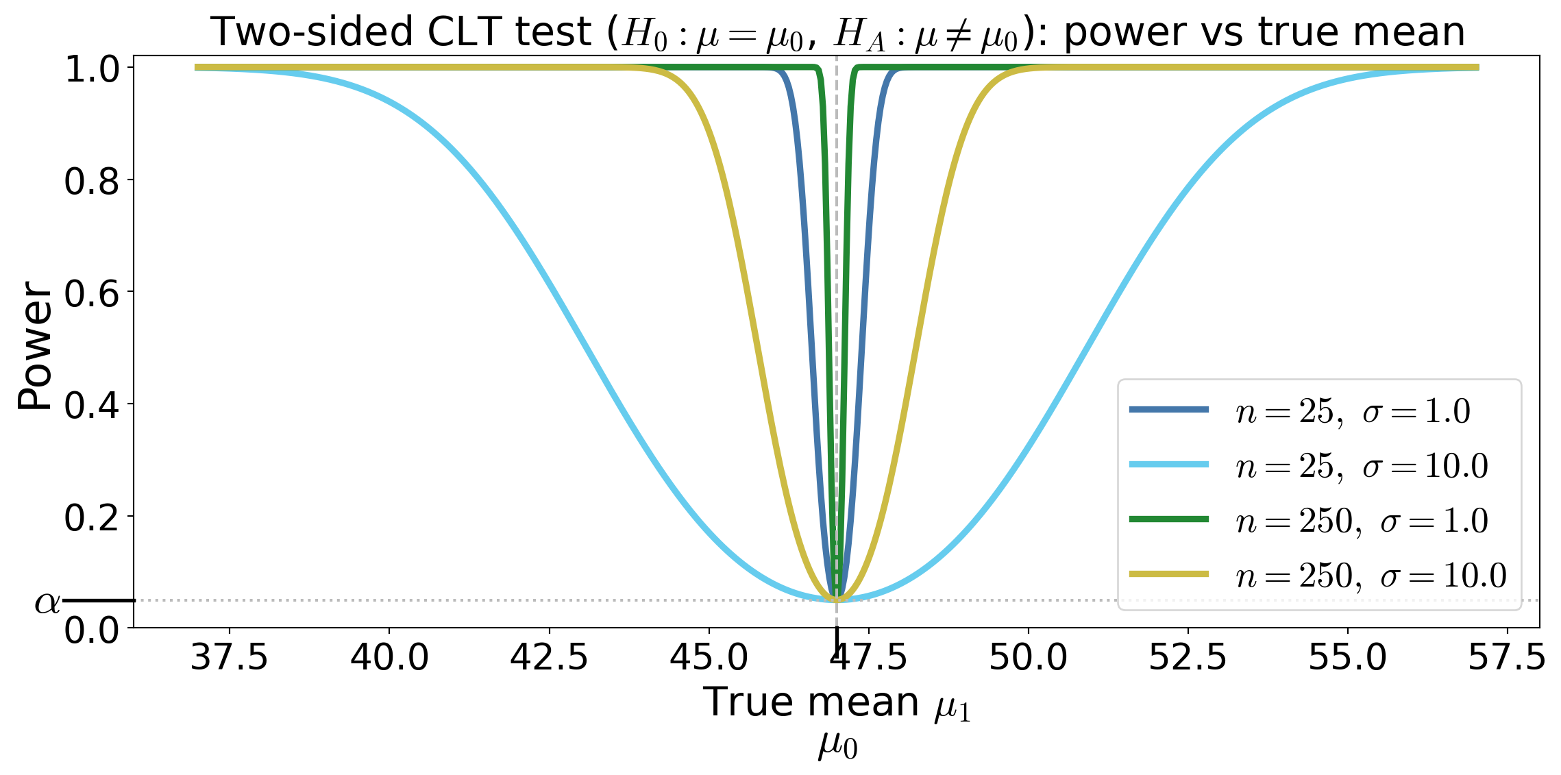
Power is \(\Prob(\text{reject} \mid \theta)\)
It is not \(\Prob(\theta \mid \text{data})\)
Power describes the test design, not the evidence in this sample
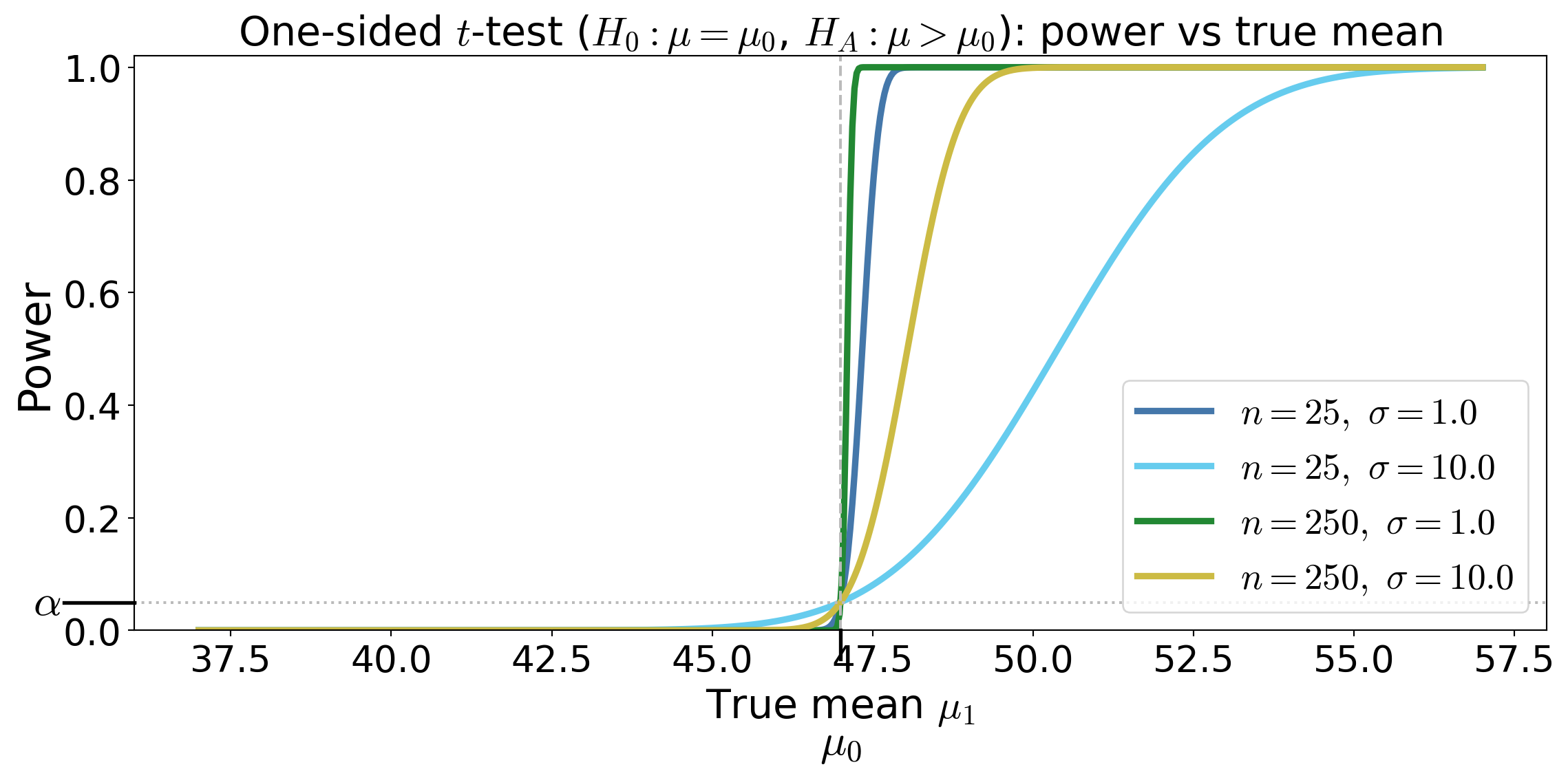
One-sided test for a mean under Normal data
Suppose \(X_1,\dots,X_n\) IID with \(X_i \sim \Norm(\mu,\sigma^2)\)
Test \(H_0: \mu \le \mu_0\) against \(H_A: \mu > \mu_0\)
Test statistic \(\displaystyle T_n(\vX) = \frac{\barX_n - \mu_0}{S_n/\sqrt{n}} \sim t_{n-1} \text{ under } \mu=\mu_0\)
Rejection region \(\RR = (t_{n-1,\alpha}, \infty)\)
Power function — the probability of rejecting \(H_0\) when the true mean is \(\mu_1\)
\[\begin{multline*} T_n(\vX) \sim t_{n-1}(\delta) \text{ for } \delta = \frac{\mu_1 - \mu_0}{\sigma/\sqrt{n}} \\ \implies \power(\mu_1) = \Prob(T_n(\vX) > t_{n-1,\alpha} \mid \mu=\mu_1) = 1 - F_{t_{n-1}(\delta)}\!\left(t_{n-1,\alpha}\right) \end{multline*}\]
where \(F_{t_{n-1}(\delta)}\) is the CDF of the noncentral t distribution with \(n-1\) degrees of freedom and noncentrality parameter \(\delta\)
- \(p\)-value for observed \(t_{\text{obs}}\) is \(p = \Prob(t_{n-1} \ge t_{\text{obs}})\)
Power curves for the one-sided \(t\)-test
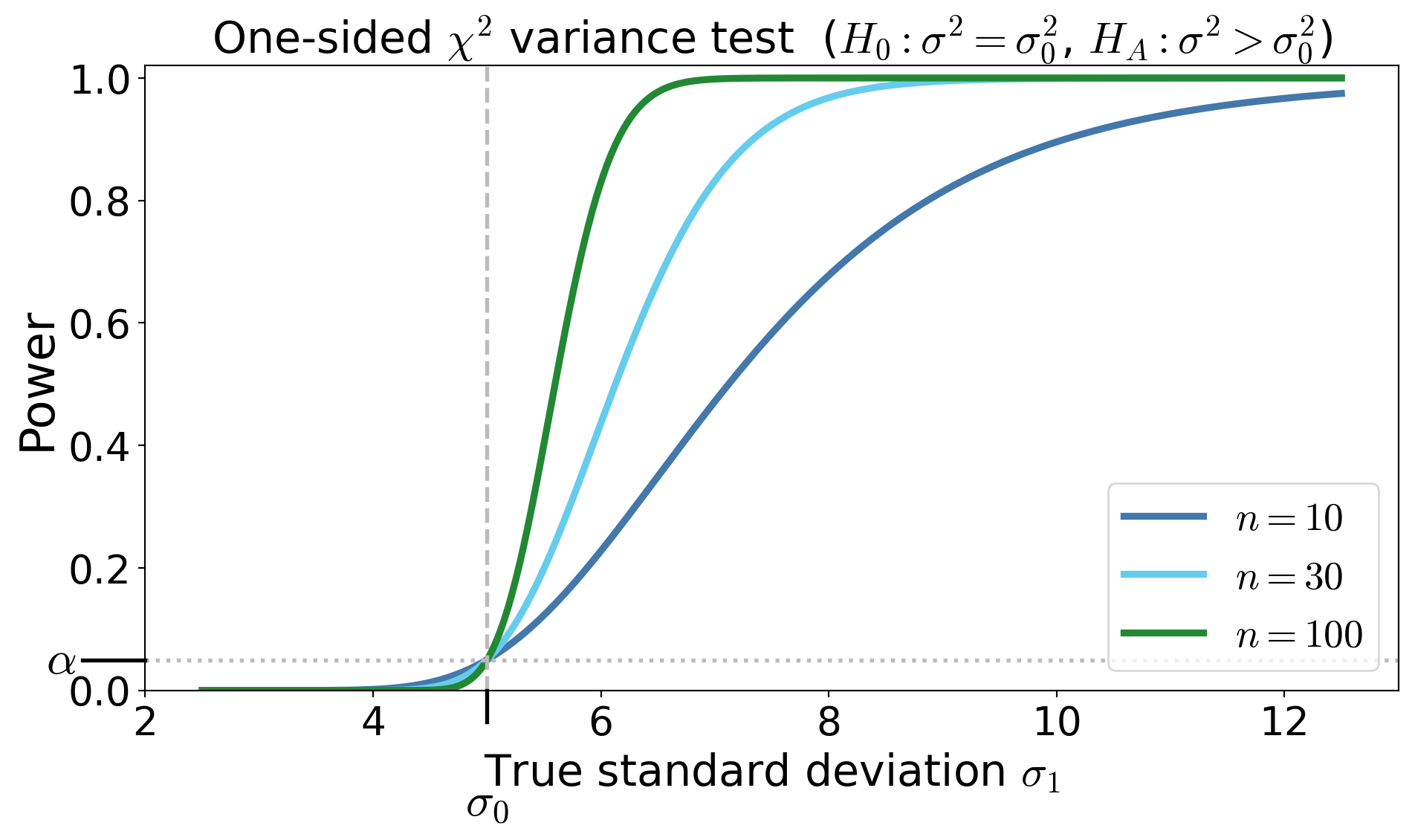
One-sided \(\chi^2\) test for the variance under Normal data
Suppose \(X_1,\dots,X_n\) IID with \(X_i \sim \Norm(\mu,\sigma^2)\).
Test \(H_0: \sigma^2 = \sigma_0^2\) against \(H_A: \sigma^2 > \sigma_0^2\)
Pivot / test statistic \(\displaystyle T_n(\vX) = \frac{(n-1)S_n^2}{\sigma_0^2} \sim \chi^2_{n-1} \text{ under } H_0\)
- where \(S_n^2\) is the unbiased sample variance
Rejection region \(\RR = (\chi^2_{n-1,\alpha}, \infty)\)
Power function
\[ \power(\sigma_1) = \Prob\!\left( T_n(\vX) > \chi^2_{n-1,\alpha}\mid \sigma = \sigma_1 \right) = \Prob\!\left( \chi^2_{n-1} > \frac{\sigma_0^2}{\sigma_1^2}\chi^2_{n-1,\alpha} \right) \]\(p\)-value for observed \(t_{\text{obs}}\) is \(p = \Prob(\chi^2_{n-1} \ge t_{\text{obs}})\)
Power curves for the one-sided \(\chi^2\) test
Try on your own
\(\exstar\)Construct small sample size one-sided and two-sided tests for the mean of an exponential distribution and sketch the power curves
Optimal Tests and Likelihood Methods
(CB §8.2–8.3; WMS §10.10-10.11)
From procedures to optimality
We have constructed tests, and we have computed their size and power, but
Among all tests with size \(\alpha\), which test has the highest power against a fixed alternative?
To compare two hypotheses
\[ H_0: \theta = \theta_0 \qquad \text{vs} \qquad H_A: \theta = \theta_A \]
Consider the likelihood ratio statistic constructed from the ratio of the likelihood values based on data \(\vX = (X_1,\dots,X_n)\): \[ \Lambda(\vX) = \frac{L(\theta_0 \mid \vX)} {L(\theta_A \mid \vX)} = \frac{\varrho_{\vX}(\vX \mid \theta_0)}{\varrho_{\vX}(\vX \mid \theta_A)} \]
If the data are much more likely under \(H_A\) than under \(H_0\), the ratio \(\Lambda(\vX)\) will be small, and this is evidence against \(H_0\)
Neyman–Pearson lemma (simple vs simple)
Test
\[ H_0:\theta=\theta_0 \qquad\text{vs}\qquad H_A:\theta=\theta_A \]
Among all tests with size \(\alpha\), the test that rejects for sufficiently small likelihood ratio is most powerful
Reject \(H_0\) when
\[ \Lambda(\vX) = \frac{L(\theta_0 \mid \vX)} {L(\theta_A \mid \vX)} < k \]
where \(k\) is chosen so that
\[ \Prob(\text{reject }H_0 \mid \theta = \theta_0)= \Prob(\Lambda(\vX) < k \mid \theta = \theta_0) = \alpha \]
A test that is most powerful for all alternatives in a class is called uniformly most powerful (UMP)
Example: mean of IID Normal data with known \(\sigma\), testing simple vs simple
\[ H_0:\mu=\mu_0 \qquad H_A:\mu=\mu_A \quad \text{with } \mu_A > \mu_0 \]
Suppose \(X_1,\dots,X_n \IIDsim \Norm(\mu,\sigma^2)\). The likelihood ratio test statistic based on this data, \(\vX = (X_1,\dots,X_n)\), is
\[ \Lambda = \frac{L(\mu_0 \mid \vX)}{L(\mu_A \mid \vX)} \]
Because the logarithm is increasing, it is convenient to work with
\[\begin{multline*} \log \Lambda(\vX) = \log \bigl(L(\mu_0 \mid \vX)\bigr)-\log L(\mu_A \mid \vX) \\ = -\frac{1}{2\sigma^2} \sum_{i=1}^n (X_i-\mu_0)^2 + \frac{1}{2\sigma^2} \sum_{i=1}^n (X_i-\mu_A)^2 = \cdots \\ = \frac{n(\mu_0-\mu_A)}{\sigma^2} \left(\barX_n - \frac{\mu_0+\mu_A}{2}\right) \end{multline*}\]
\[\begin{equation*} \log \Lambda(\vX) = \frac{n(\mu_0-\mu_A)}{\sigma^2} \left(\barX_n - \frac{\mu_0+\mu_A}{2}\right) \end{equation*}\]
Reject when \(\barX_n > c\) for some cut-off \(c\), which is chosen so that
\[ \Prob(\barX_n>c \mid \mu=\mu_0)=\alpha, \qquad \text{i.e., } c = \mu_0 + z_\alpha \frac{\sigma}{\sqrt n} \]
Because the Type-I error is computed assuming \(H_0\) is true, the cutoff does not depend on \(\mu_A\)
The likelihood ratio test is most powerful among all tests with size \(\alpha\) for testing \(H_0: \mu = \mu_0\) vs \(H_A: \mu = \mu_A\) with \(\mu_A > \mu_0\) when \(\sigma\) is known
The likelihood ratio test therefore reproduces the classical \(z\)-test for the mean of a normal distribution with known variance
From Neyman–Pearson to likelihood ratio tests for composite hypotheses
More generally, for hypotheses
\[ H_0:\theta \in \ct_0 \qquad\text{vs}\qquad H_A:\theta \in \ct_A \]
the likelihood ratio statistic based on data \(\vX = (X_1,\dots,X_n)\) is
\[ \Lambda(\vX) = \frac{\sup_{\theta\in \ct_0} L(\theta \mid \vX)} {\sup_{\theta\in \ct} L(\theta \mid \vX)} =\frac{\text{best fit under }H_0} {\text{best fit over the entire parameter space}} \]
- The numerator is the largest likelihood under \(H_0\)
- The denominator is the largest likelihood over the entire parameter space
Reject for small \(\Lambda\)
Example: mean of IID Normal data with known \(\sigma\), testing simple vs composite (two-sided)
\[ H_0:\mu=\mu_0 \qquad H_A:\mu\ne \mu_0 \]
Suppose \(X_1,\dots,X_n \IIDsim \Norm(\mu,\sigma^2)\). The likelihood ratio test statistic is
\[ \Lambda(\vX) = \frac{\sup_{\mu=\mu_0} L(\mu \mid \vX)} {\sup_{\mu\in\reals} L(\mu \mid \vX)} = \frac{L(\mu_0 \mid \vX)}{L(\barX_n \mid \vX)}, \qquad \text{since the MLE of $\mu$ is $\barX_n$ for IID normal data} \]
Because the logarithm is increasing, it is convenient to work with
\[\begin{multline*} \log \Lambda(\vX) = \log L(\mu_0 \mid \vX)-\log L(\barX_n \mid \vX) \\ = -\frac{1}{2\sigma^2}\sum_{i=1}^n (X_i-\mu_0)^2 +\frac{1}{2\sigma^2}\sum_{i=1}^n (X_i-\barX_n)^2 = \cdots = -\frac{n}{2\sigma^2}(\barX_n-\mu_0)^2 \end{multline*}\]
\[\begin{equation*} \log \Lambda(\vX) = -\frac{n}{2\sigma^2}(\barX_n-\mu_0)^2 \end{equation*}\]
Reject when \(\Lambda(\vX)\) is small \(\iff |\barX_n-\mu_0|\) is large, equivalently, reject when
\[ \left|\frac{\barX_n-\mu_0}{\sigma/\sqrt n}\right| > z_{\alpha/2} \]
The cutoff is chosen so that
\[ \Prob\!\left(\left|\frac{\barX_n-\mu_0}{\sigma/\sqrt n}\right|>z_{\alpha/2}\ \middle|\ \mu=\mu_0\right)=\alpha, \]
which depends only on \(\mu_0\), \(\sigma\), \(n\), and \(\alpha\)
The likelihood ratio test therefore reproduces the classical two-sided \(z\)-test for the mean of a normal distribution with known variance
Example: LRT for a normal mean (unknown variance) — nuisance parameters
\[ H_0:\mu=\mu_0 \qquad \text{vs} \qquad H_A:\mu\ne\mu_0 \]
Suppose \(X_1,\dots,X_n \IIDsim \Norm(\mu,\sigma^2)\)
Parameter vector: \(\theta=(\mu,\sigma^2), \qquad \sigma^2\) is a nuisance parameter
Step 1: Unrestricted MLE
Log-likelihood: \[ \ell(\mu,\sigma^2) = -\frac{n}{2}\log (\sigma^2) - \frac{1}{2\sigma^2} \sum_{i=1}^n (X_i-\mu)^2 + \text{constants} \]
Maximizing gives \[\begin{gather*} \mu_{\MLE} = \barX_n, \qquad \sigma_{\MLE}^2 = \frac{1}{n}\sum_{i=1}^n (X_i-\barX_n)^2 = \frac{n-1}{n} S_n^2 \\ \sup_{\mu,\sigma^2} \ell(\mu,\sigma^2) = -\frac{n}{2}\log (\sigma^2_{\MLE}) - \frac{n}{2} + \text{constants} \end{gather*}\]
Step 2: MLE under \(H_0\)
Under \(\mu=\mu_0\), \[\begin{gather*} \sigma_{0,\MLE}^2 = \frac{1}{n}\sum_{i=1}^n (X_i-\mu_0)^2 = (\barX_n - \mu_0)^2 + \frac 1n \sum_{i=1}^n (X_i-\barX_n)^2 = (\barX_n - \mu_0)^2 + \sigma_{\MLE}^2 \\ \sup_{\sigma^2} \ell(\mu_0,\sigma^2) = -\frac{n}{2}\log (\sigma^2_{0,\MLE}) - \frac{n}{2} + \text{constants} \end{gather*}\]
Step 3: (Log) likelihood ratio
\[\begin{gather*} \log \bigl(\Lambda(\vX) \bigr) = \sup_{\sigma^2} \ell(\mu_0,\sigma^2_{0,\MLE}) - \sup_{\mu,\sigma^2} \ell(\mu,\sigma^2_{\MLE}) = -\frac{n}{2}\log (\sigma^2_{0,\MLE}) + \frac{n}{2}\log (\sigma^2_{\MLE}) \\ \Lambda(\vX) = \left(\frac{\sigma^2_{0,\MLE}}{\sigma^2_{\MLE}}\right)^{-n/2} \end{gather*}\]
Step 4: Where nuisance disappears
Therefore \[\begin{align*} \frac{\sigma_{0,\MLE}^2}{\sigma_{\MLE}^2} & = \frac{(\barX_n - \mu_0)^2 + \sigma_{\MLE}^2}{\sigma_{\MLE}^2} = \frac{(\barX_n-\mu_0)^2} {(n-1) S_n^2/n} + 1 = \frac{T_n^2}{n-1} + 1\\ \Lambda(\vX) & = \left( 1 + \frac{T_n^2}{n-1} \right)^{-n/2} \end{align*}\]
where \(\displaystyle T_n = \frac{\barX_n-\mu_0}{S/\sqrt n}\) is the familiar \(t\)-statistic
The likelihood ratio depends only on the \(t\)-statistic for testing \(H_0: \mu = \mu_0\) vs \(H_A: \mu \ne \mu_0\)
The nuisance parameter \(\sigma^2\) has disappeared
\(\exstar\) Show that the LRT for testing \(H_0: \mu = \mu_0\) vs \(H_A: \mu = \mu_1\) with \(\mu_1 > \mu_0\) and \(\sigma\) unknown is the familar one-sided \(t\)-test as
Wilks’ Theorem
\[ \Lambda(\vX) = \frac{\displaystyle \sup_{\theta\in \ct_0} L(\theta \mid \vX)} {\displaystyle \sup_{\theta\in \ct} L(\theta \mid \vX)} \]
Under regularity conditions,
\[ -2 \log \Lambda \dto \chi^2_{\df} \] where the degrees of freedom is \[ \df = \dim(\text{full model}) - \dim(\text{null model}) \]
Example: Normal data with unknown \(\sigma\)
- Full model for \(\Norm(\mu,\sigma^2)\) has \(\dim(\ct) = 2\)
- Null model for \(H_0: \mu = \mu_0\) has \(\dim(\ct_0) = 1\)
- \(\df = 2 - 1 = 1\)
Why bother with the likelihood ratio test (LRT)
\[ \Lambda(\vX) = \frac{\sup_{\theta \in \ct_0} L(\theta \mid \vX)} {\sup_{\theta \in \ct} L(\theta \mid \vX)} \qquad \text{Reject when $\Lambda(\vX)$ is small} \]
Even though
We already know the \(z\), \(t\), and other tests
We still need to choose the rejection region cut-off to get the desired size \(\alpha\)
However, the LRT
Is a unifying concept
Handles composite hypotheses
Reproduces \(z\), \(t\), \(\chi^2\), \(F\) tests
Scales to multi-parameter models
Has large-sample theory (Wilks)
\(\exstar\) WMS 10.105, 10.106, 10.112
\(\exstar\) CB 8.29, 8.40, 8.41
© 2026 Fred J. Hickernell · Illinois Tech · assisted by ChatGPT · Hypothesis Testing · MATH 476 — Statistics Website · \(\exstar\) = exercise