MATH 332 — Fall 2026

Special Topics
Anton, Rorres, & Kaul Selected Chs. 7–10
FFT and tensor enrichment

Fred J. Hickernell

October 9, 2026

Course Map

Course decks

• Why Linear Algebra?
• Systems and Matrices
• Inverses
• Matrix Transformations
• Determinants
• Euclidean Spaces
• Vector Spaces and Span
• Bases and Coordinates
• Matrix Spaces and Rank
• Eigenvalues
• Inner Products
• Special Topics

In this deck

Choose coordinates that expose structure

\(\mat{A}=\mat{U}_r\mat{\Sigma}_r\mat{V}_r^{\mathsf T}\)

• Singular Value Decomposition
• Regression Through QR and SVD
• Quadratic Forms and Principal Axes
• Fourier Coordinates and the FFT
• Tensor Products and Structured Data
• Networks and Iterative Eigenvectors
• Big Ideas

Instructor draft: modular sections, not a commitment to cover every topic. SVD and regression are the priority. QR/least squares and complex inner products are drafted in Inner Product Spaces (Anton §§6.3–6.6); review and teach that foundation first. Quadratic forms can precede SVD if the spectral theorem needs development first. FFT and tensors supplement Anton; networks and iterative eigenvectors are optional. Suggested demonstrations remain to be built, not linked as existing notebooks.

Which topics would you like to explore?

SVD and its regression connection are our priority

Rank your next two choices and give a question or application you want to explore

• Quadratic forms and principal axes
• Fourier transforms and FFT
• Tensors and structured images
• Power iteration and PageRank
• Graph Laplacians and networks

Selections depend on class interest and remaining time

Ask for an informal show of hands or a short ranked response in class. No external poll has been created. Treat preferences as guidance for optional coverage, not a promise to cover everything.

Singular Value Decomposition

• What can a rectangular matrix do?
• The SVD separates directions from scale
• Each singular direction has its own stretch
• A worked SVD without square roots of large matrices
• See the singular stretches
• Why an SVD exists
• The four spaces reappear in orthonormal coordinates
• A matrix is a sum of rank-one maps
• The best low-rank approximation has a measurable error
• Practice reading singular values

What can a rectangular matrix do?

\(\mat{A}:\reals^n\to\reals^m\) may stretch, turn, and collapse directions

Eigenvectors require a square matrix; singular vectors work for every shape

Choose orthonormal input and output directions adapted to the map

The SVD separates directions from scale

For a real \(m\times n\) matrix of rank \(r>0\): \[\begin{gather*} \mat{A}=\mat{U}_r\mat{\Sigma}_r\mat{V}_r^{\mathsf T},\qquad \mat{\Sigma}_r=\operatorname{diag}(\sigma_1,\ldots,\sigma_r)\\ \sigma_1\ge\cdots\ge\sigma_r>0,\qquad \mat{U}_r^{\mathsf T}\mat{U}_r=\mat{V}_r^{\mathsf T}\mat{V}_r=\mat{I}_r \end{gather*}\]

Factor	Shape	Role
\(\mat{V}_r^{\mathsf T}\)	\(r\times n\)	input coordinates
\(\mat{\Sigma}_r\)	\(r\times r\)	stretch each coordinate
\(\mat{U}_r\)	\(m\times r\)	assemble the output

This is the compact SVD. The zero matrix has no positive singular values and an empty compact factorization; its pseudoinverse is zero. Orthogonal completions give the full SVD with U m-by-m, V n-by-n, and rectangular Sigma.

Each singular direction has its own stretch

Write \(\vct{U}_j\) and \(\vct{V}_j\) for columns of the compact factors \[\begin{gather*} \mat{A}\vct{V}_j=\sigma_j\vct{U}_j,\qquad \mat{A}^{\mathsf T}\vct{U}_j=\sigma_j\vct{V}_j\\ \mat{A}\vct{x}=\sum_{j=1}^r\sigma_j\vct{U}_j \bigl(\vct{V}_j^{\mathsf T}\vct{x}\bigr) \end{gather*}\]

Input perpendicular to every \(\vct{V}_j\) is sent to zero

Singular values measure stretches, not signed eigenvalues

A worked SVD without square roots of large matrices

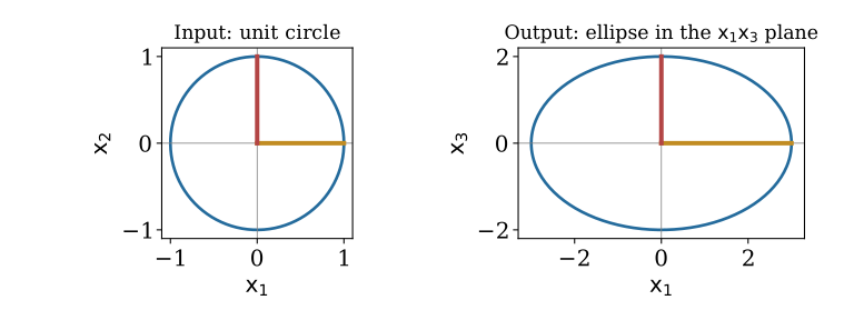
\[\begin{gather*} \mat{A}=\begin{pmatrix}3&0\\0&0\\0&2\end{pmatrix},\quad \mat{U}_r=\begin{pmatrix}1&0\\0&0\\0&1\end{pmatrix},\quad \mat{\Sigma}_r=\begin{pmatrix}3&0\\0&2\end{pmatrix},\quad \mat{V}_r=\mat{I}_2\\ \mat{A}\begin{pmatrix}\cos t\\\sin t\end{pmatrix} =\begin{pmatrix}3\cos t\\0\\2\sin t\end{pmatrix} \end{gather*}\]

The unit circle becomes an ellipse in the \(x_1x_3\) plane

The ellipse axes are the left singular vectors; their lengths are the singular values

See the singular stretches

Why an SVD exists

\(\mat{A}^{\mathsf T}\mat{A}\) is symmetric and positive semidefinite \[\begin{gather*} \vct{x}^{\mathsf T}\mat{A}^{\mathsf T}\mat{A}\vct{x} =\|\mat{A}\vct{x}\|^2\ge0\\ \mat{A}^{\mathsf T}\mat{A}\vct{V}_j=\sigma_j^2\vct{V}_j,\qquad \vct{U}_j=\frac{\mat{A}\vct{V}_j}{\sigma_j}\quad(\sigma_j>0) \end{gather*}\]

Orthogonal eigenvectors on the input side produce orthonormal output vectors

For positive singular values, U_i^T U_j = V_i^T A^T A V_j/(sigma_i sigma_j) = delta_ij. Use the real symmetric spectral theorem, developed in the quadratic-forms section. This is an existence argument, not a recommended numerical algorithm: forming A^T A squares the full-column-rank condition number.

The four spaces reappear in orthonormal coordinates

Space	SVD description
\(\operatorname{col}(\mat{A})\)	span of \(\vct{U}_1,\ldots,\vct{U}_r\)
\(\operatorname{row}(\mat{A})\)	span of \(\vct{V}_1,\ldots,\vct{V}_r\)
\(\operatorname{null}(\mat{A})\)	perpendicular to all \(\vct{V}_j\)
\(\operatorname{null}(\mat{A}^{\mathsf T})\)	perpendicular to all \(\vct{U}_j\)

Complete the columns of \(\mat{U}_r\) and \(\mat{V}_r\) to orthonormal bases to obtain bases of the two null spaces

Recall matrix spaces

A matrix is a sum of rank-one maps

\[\begin{equation*} \mat{A}=\sum_{j=1}^r\sigma_j\vct{U}_j\vct{V}_j^{\mathsf T} \end{equation*}\]

Each term reads one input coordinate and sends it along one output direction

Keep only the first \(k\) terms: \[\begin{equation*} \mat{A}_k=\sum_{j=1}^k\sigma_j\vct{U}_j\vct{V}_j^{\mathsf T},\qquad 0\le k<r \end{equation*}\]

A controlled approximation using fewer directions

The best low-rank approximation has a measurable error

Define \(\|\mat{B}\|_F^2=\sum_{i,j}|b_{ij}|^2\) and \(\|\mat{B}\|_2=\max_{\|\vct{x}\|=1}\|\mat{B}\vct{x}\|\) \[\begin{gather*} \|\mat{A}-\mat{A}_k\|_2=\sigma_{k+1}\\ \|\mat{A}-\mat{A}_k\|_F^2=\sum_{j=k+1}^r\sigma_j^2 \end{gather*}\]

\(\mat{A}_k\) minimizes either error over matrices of rank at most \(k\)

Choose the rank by the accuracy needed, not only by the appearance of the image

Eckart–Young–Mirsky theorem; statement without proof. Approximation need not be unique when singular values tie. For an m-by-n grayscale image, storing compact factors uses k(m+n+1) scalar entries instead of mn, before file-format overhead or quantization.

Practice reading singular values

\(\exstar\) A matrix has singular values \(8,3,1\)
Find the rank-one spectral error and rank-two Frobenius error
How many rank-one terms reproduce the matrix exactly?

Answers: 3; 1; three terms. Distinguish the two error norms.

Regression Through QR and SVD

• Regression asks for the closest attainable data
• QR solves full-column-rank least squares
• The pseudoinverse reverses the nonzero stretches
• Rank deficiency changes coefficients, not the fitted vector
• A regression example with a redundant feature
• Small singular values amplify data perturbations
• Truncation and ridge control small stretches
• Which factorization serves the regression question?
• Practice separating fit from coefficients

Regression asks for the closest attainable data

Fit observations \(b_i\) using features \(a_{ij}\) and coefficients \(x_j\) \[\begin{gather*} \widehat{\vct{b}}=\mat{A}\widehat{\vct{x}},\qquad \widehat{\vct{x}}\in\arg\min_{\vct{x}}\|\mat{A}\vct{x}-\vct{b}\|^2\\ \mat{A}^{\mathsf T}(\vct{b}-\widehat{\vct{b}})=\vct{0} \end{gather*}\]

\(\widehat{\vct{b}}\) is the orthogonal projection onto \(\operatorname{col}(\mat{A})\)

A column of ones supplies an intercept

Prerequisite: inner products and least squares

QR solves full-column-rank least squares

For \(m\ge n\) and independent columns: \[\begin{gather*} \mat{A}=\mat{Q}\mat{R},\quad \mat{Q}^{\mathsf T}\mat{Q}=\mat{I}_n,\quad \mat{R}\text{ upper triangular and invertible}\\ \|\mat{A}\vct{x}-\vct{b}\|^2 =\|\mat{R}\vct{x}-\mat{Q}^{\mathsf T}\vct{b}\|^2 +\|(\mat{I}_m-\mat{Q}\mat{Q}^{\mathsf T})\vct{b}\|^2\\ \mat{R}\widehat{\vct{x}}=\mat{Q}^{\mathsf T}\vct{b} \end{gather*}\]

Compute orthogonal coordinates, then use back substitution

Reduced QR: Q is m-by-n, R is n-by-n. This R is the triangular QR factor, different from R in A=C R; reused matrix letters are defined by the current factorization. Gram–Schmidt explains the factorization; Householder QR is the standard practical method. Full development belongs in Anton §6.3 in Inner Product Spaces; this is a refresher.

The pseudoinverse reverses the nonzero stretches

\[\begin{gather*} \mat{A}^{\dagger}=\mat{V}_r\mat{\Sigma}_r^{-1}\mat{U}_r^{\mathsf T}\\ \widehat{\vct{x}}=\mat{A}^{\dagger}\vct{b} =\sum_{j=1}^r\frac{\vct{U}_j^{\mathsf T}\vct{b}}{\sigma_j}\vct{V}_j\\ \widehat{\vct{b}}=\mat{A}\widehat{\vct{x}} =\mat{U}_r\mat{U}_r^{\mathsf T}\vct{b} \end{gather*}\]

Works for rectangular and rank-deficient matrices

The pseudoinverse selects the least-squares solution with smallest Euclidean norm

Rank deficiency changes coefficients, not the fitted vector

Every least-squares minimizer has the form \[\begin{equation*} \vct{x}=\mat{A}^{\dagger}\vct{b}+\vct{z},\qquad \vct{z}\in\operatorname{null}(\mat{A}) \end{equation*}\]

• All give the same fitted vector \(\widehat{\vct{b}}\)
• The pseudoinverse solution lies in \(\operatorname{row}(\mat{A})\)
• Adding a perpendicular null-space component increases the coefficient norm

Use the orthogonal splitting R^n = row(A) plus null(A). The minimizer is unique exactly when A has full column rank. This also covers underdetermined consistent systems.

A regression example with a redundant feature

\[\begin{gather*} \mat{A}=\begin{pmatrix}1&1\\1&1\end{pmatrix},\quad \vct{b}=\begin{pmatrix}2\\4\end{pmatrix},\quad \vct{U}_1=\vct{V}_1=\frac1{\sqrt2}\begin{pmatrix}1\\1\end{pmatrix},\quad\sigma_1=2\\ \widehat{\vct{x}}=\begin{pmatrix}3/2\\3/2\end{pmatrix},\quad \widehat{\vct{b}}=\begin{pmatrix}3\\3\end{pmatrix},\quad \vct{b}-\widehat{\vct{b}}=\begin{pmatrix}-1\\1\end{pmatrix} \end{gather*}\]

Both features are identical: only \(x_1+x_2=3\) is identifiable

The smallest-norm solution divides the total equally

Small singular values amplify data perturbations

A perturbation \(\delta\vct{b}\) changes the pseudoinverse coefficients by \[\begin{equation*} \delta\widehat{\vct{x}} =\sum_{j=1}^r\frac{\vct{U}_j^{\mathsf T}\delta\vct{b}}{\sigma_j}\vct{V}_j \end{equation*}\]

Small positive \(\sigma_j\): large coefficient changes in direction \(\vct{V}_j\)

For full column rank, \(\kappa_2(\mat{A})=\sigma_1/\sigma_n\)

An accurate fit can coexist with poorly determined coefficients

Keep rank and conditioning distinct. Exact zero singular values create nonidentifiability; small positive ones create sensitivity. Feature scaling affects these values and the meaning of a coefficient-norm penalty.

Truncation and ridge control small stretches

Truncated SVD retains only singular values above a chosen threshold \(\tau\): \[\begin{equation*} \widehat{\vct{x}}_\tau =\sum_{\sigma_j>\tau}\frac{\vct{U}_j^{\mathsf T}\vct{b}}{\sigma_j}\vct{V}_j \end{equation*}\]

Ridge minimizes \(\|\mat{A}\vct{x}-\vct{b}\|^2+\lambda\|\vct{x}\|^2\), \(\lambda>0\): \[\begin{equation*} \widehat{\vct{x}}_\lambda =\sum_{j=1}^r\frac{\sigma_j}{\sigma_j^2+\lambda} (\vct{U}_j^{\mathsf T}\vct{b})\vct{V}_j \end{equation*}\]

Truncation discards directions; ridge shrinks their contributions

This ridge formula penalizes every coefficient, including an intercept if present. In typical regression, center features and response or explicitly exempt the intercept; then the formula must be applied to the corresponding centered or weighted-penalty problem. Parameter choice requires a noise model or validation data; this deck introduces the algebra only.

Which factorization serves the regression question?

Question	Useful tool
Full-column-rank least-squares coefficients	QR and a triangular solve
Rank deficiency and minimum-norm coefficients	SVD and pseudoinverse
Sensitivity and numerical rank	Singular values and feature scaling
Noise-sensitive directions	Truncation or ridge

Forming \(\mat{A}^{\mathsf T}\mat{A}\) squares \(\kappa_2(\mat{A})\) when \(\mat{A}\) has full column rank

Prefer an orthogonal factorization to explicitly inverting the normal-equation matrix

Practice separating fit from coefficients

\(\exstar\) For the redundant-feature example, describe every least-squares solution
Verify that the residual is perpendicular to both columns
Explain why \((3/2,3/2)^{\mathsf T}\) has the smallest norm

Solutions: \((3/2+t,3/2-t)^{\mathsf T}\), t real. Each column dotted with (-1,1)^T is zero. Squared coefficient norm is 9/2+2t^2, minimized at t=0.

Quadratic Forms and Principal Axes

• Symmetry gives orthogonal eigenvectors
• A tilted ellipse becomes an axis-aligned ellipse
• See the principal axes
• Signs distinguish bowls from saddles
• Practice finding the principal directions

Symmetry gives orthogonal eigenvectors

For a real symmetric matrix: \[\begin{gather*} \mat{A}=\mat{Q}\mat{\Lambda}\mat{Q}^{\mathsf T},\qquad \mat{Q}^{\mathsf T}\mat{Q}=\mat{I}\\ \vct{x}=\mat{Q}\vct{y}\implies \vct{x}^{\mathsf T}\mat{A}\vct{x}=\sum_j\lambda_j y_j^2 \end{gather*}\]

The real symmetric spectral theorem: an orthonormal eigenbasis always exists

Principal-axis coordinates remove mixed terms

Distinct eigenvalues yield perpendicular eigenvectors; repeated eigenspaces admit orthonormal bases. State the spectral theorem without a full proof at this introductory level.

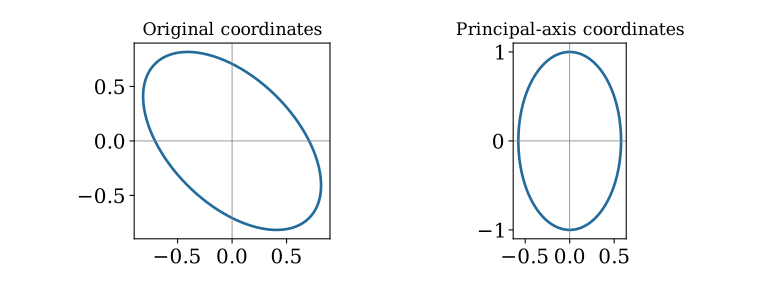
A tilted ellipse becomes an axis-aligned ellipse

\[\begin{gather*} \mat{A}=\begin{pmatrix}2&1\\1&2\end{pmatrix},\quad \mat{Q}=\frac1{\sqrt2}\begin{pmatrix}1&1\\1&-1\end{pmatrix},\quad \mat{\Lambda}=\begin{pmatrix}3&0\\0&1\end{pmatrix}\\ 2x_1^2+2x_1x_2+2x_2^2=1 \quad\longleftrightarrow\quad 3y_1^2+y_2^2=1 \end{gather*}\]

Semiaxis lengths: \(1/\sqrt3\) and \(1\)

Eigenvectors give the axes; eigenvalues determine the curvature

See the principal axes

Signs distinguish bowls from saddles

For symmetric \(\mat{A}\):

Eigenvalues	Quadratic form \(\vct{x}^{\mathsf T}\mat{A}\vct{x}\)
All positive	positive definite: positive for every \(\vct{x}\ne\vct{0}\)
All nonnegative	positive semidefinite: never negative
Positive and negative	indefinite: changes sign

Least-squares curvature: \(\mat{A}^{\mathsf T}\mat{A}\)

Ridge curvature: \(\mat{A}^{\mathsf T}\mat{A}+\lambda\mat{I}\), positive definite for \(\lambda>0\)

Practice finding the principal directions

\(\exstar\) Find orthonormal eigenvectors of \(\begin{pmatrix}2&-1\\-1&2\end{pmatrix}\)
Use them to rewrite \(2x_1^2-2x_1x_2+2x_2^2\)
Is this form positive definite?

The vector (1,1)^T/sqrt(2) has eigenvalue 1; (1,-1)^T/sqrt(2) has eigenvalue 3. In that ordered eigenbasis the form is y_1^2+3y_22, hence positive definite.

Fourier Coordinates and the FFT

• Sampled signals are vectors
• Fourier directions are orthogonal over the complex field
• Four samples give a concrete Fourier calculation
• The FFT reuses the even and odd calculations
• Convolution becomes componentwise multiplication
• Practice recognizing frequency directions

Sampled signals are vectors

A signal sampled at \(n\) equally spaced points becomes \(\vct{x}\in\mathbb{C}^n\)

Index samples and frequencies by \(0,\ldots,n-1\) \[\begin{gather*} \omega_n=e^{-2\pi\sqrt{-1}/n},\qquad (\mat{F}_n)_{kj}=\omega_n^{kj}\\ \vct{X}=\mat{F}_n\vct{x},\qquad \vct{x}=\frac1n\mat{F}_n^*\vct{X} \end{gather*}\]

\(\mat{B}^*=\overline{\mat{B}}^{\mathsf T}\) denotes the conjugate transpose

Frequency coordinates reveal oscillations hidden in the sample values

Fourier directions are orthogonal over the complex field

Use \(\langle\vct{u},\vct{v}\rangle=\vct{u}^*\vct{v}\) \[\begin{equation*} \sum_{j=0}^{n-1}\omega_n^{(k-\ell)j} =\begin{cases}n,&k=\ell\\0,&k\ne\ell\end{cases} \end{equation*}\]

Thus \(\mat{F}_n^*\mat{F}_n=n\mat{I}_n\) and \(\mat{F}_n/\sqrt n\) is unitary

The DFT is a scaled change to an orthonormal basis

Frequency indices are in 0,…,n-1. For unequal indices, use the finite geometric series; omega_n^(k-l) is not 1. The inverse basis vectors use positive exponents, consistent with the earlier continuous Fourier convention. Distinguish a complex inner product from an ordinary transpose product.

Four samples give a concrete Fourier calculation

\[\begin{gather*} \mat{F}_4=\begin{pmatrix} 1&1&1&1\\1&-\sqrt{-1}&-1&\sqrt{-1}\\ 1&-1&1&-1\\1&\sqrt{-1}&-1&-\sqrt{-1} \end{pmatrix}\\ \vct{x}=\begin{pmatrix}1\\0\\-1\\0\end{pmatrix} \implies\vct{X}=\begin{pmatrix}0\\2\\0\\2\end{pmatrix} \end{gather*}\]

A real cosine uses a pair of opposite frequency directions

For real data X_(n-k) is the conjugate of X_k, with indices modulo n. The frequencies 1 and 3 for n=4 correspond to +1 and -1 cycles per record, not two unrelated physical oscillations.

The FFT reuses the even and odd calculations

For even \(n\), split \(x_0,x_2,\ldots\) from \(x_1,x_3,\ldots\)

Let \(E_k\) and \(O_k\) be their length-\(n/2\) DFTs \[\begin{align*} X_k&=E_k+\omega_n^k O_k\\ X_{k+n/2}&=E_k-\omega_n^k O_k,\qquad 0\le k<n/2 \end{align*}\]

For \(n=2^p\), repeat the split down to one-sample transforms \[\begin{equation*} T(n)=2T(n/2)+O(n)=O(n\log n) \end{equation*}\]

The FFT computes the same DFT through a sparse recursive factorization

Convolution becomes componentwise multiplication

Circular convolution of length-\(n\) vectors: \[\begin{gather*} y_j=\sum_{\ell=0}^{n-1}h_\ell x_{(j-\ell)\bmod n}\\ \mat{F}_n\vct{y}=(\mat{F}_n\vct{h})\odot(\mat{F}_n\vct{x}) \end{gather*}\]

\(\odot\): multiply matching coordinates

A circulant filter is diagonal in Fourier coordinates

Zero-pad to at least \(n_x+n_h-1\) samples to compute ordinary finite linear convolution

Interpret boundary assumptions: circular convolution wraps the signal. Arbitrary frequency truncation may cause ringing; the purpose here is to show the linear algebra, not promise universal denoising.

Practice recognizing frequency directions

\(\exstar\) Compute the DFT of \((1,1,1,1)^{\mathsf T}\) and \((1,-1,1,-1)^{\mathsf T}\)
Which is constant and which alternates?
Why does the FFT leave these answers unchanged?

Answers: (4,0,0,0)^T and (0,0,4,0)^T. Frequencies 0 and 2. FFT changes the computation, not the linear transformation.

Tensor Products and Structured Data

• An outer product separates two directions
• A tensor has coordinates after choosing bases
• Kronecker products apply maps to both factors
• Transform an image along rows and columns
• More indices describe more modes
• Practice spotting separability

An outer product separates two directions

\[\begin{gather*} \vct{u}=\begin{pmatrix}1\\2\end{pmatrix},\quad \vct{v}=\begin{pmatrix}3\\4\\5\end{pmatrix},\qquad \vct{u}\vct{v}^{\mathsf T}=\begin{pmatrix}3&4&5\\6&8&10\end{pmatrix}\\ a_{ij}=u_i v_j \end{gather*}\]

One pattern down the rows, one across the columns

A nonzero outer product has rank one

SVD builds matrices by summing such separated patterns

A tensor has coordinates after choosing bases

For finite-dimensional real spaces \(V\) and \(W\) with bases \(\{\vct{e}_i\}\) and \(\{\vct{f}_j\}\): \[\begin{gather*} V\otimes W\text{ has basis }\{\vct{e}_i\otimes\vct{f}_j\}_{i,j}\\ T=\sum_{i,j}t_{ij}\vct{e}_i\otimes\vct{f}_j,\qquad \dim(V\otimes W)=\dim(V)\dim(W) \end{gather*}\]

\(\otimes\) is bilinear; a general tensor is a sum of elementary tensors

The elementary tensor \(\vct{u}\otimes\vct{v}\) has coordinate matrix \(\vct{u}\vct{v}^{\mathsf T}\)

The coordinate array uses the listed orders of the chosen bases

This is an introductory finite-dimensional description. Tensor products can be characterized by a universal property for bilinear maps; defer that abstraction. V tensor W is not canonically the space of maps W to V: that identification uses W’s dual, or an explicitly chosen inner product. Avoid equating every two-index tensor with a linear operator without this distinction.

Kronecker products apply maps to both factors

For matrices \(\mat{B}\) and \(\mat{C}\): \[\begin{gather*} \mat{B}\otimes\mat{C}=[b_{ij}\mat{C}]_{i,j}\\ (\mat{B}\otimes\mat{C})(\vct{u}\otimes\vct{v}) =(\mat{B}\vct{u})\otimes(\mat{C}\vct{v}) \end{gather*}\]

If \(\mat{B}\) is \(p\times m\) and \(\mat{C}\) is \(q\times n\), their Kronecker product is \(pq\times mn\)

Here the coordinate vector for \(\vct{u}\otimes\vct{v}\) lists one block \(u_i\vct{v}\) per \(i\)

The ordering of tensor-product coordinates matters. This block convention agrees with NumPy kron(u,v). The next slide separately specifies column stacking for vectorization; there is no implicit claim that these two listings use the same order.

Transform an image along rows and columns

For an \(m\times n\) image matrix \(\mat{X}\): \[\begin{gather*} \mat{Y}=\mat{B}\mat{X}\mat{C}^{\mathsf T}\\ \operatorname{vec}(\mat{Y})=(\mat{C}\otimes\mat{B})\operatorname{vec}(\mat{X}) \end{gather*}\]

\(\operatorname{vec}\) stacks columns; \(\mat{B}\) acts on row indices and \(\mat{C}\) on column indices

Two-dimensional DFT: \(\mat{Y}=\mat{F}_m\mat{X}\mat{F}_n^{\mathsf T}\)

Apply the smaller transforms separately instead of building a giant Kronecker matrix

More indices describe more modes

An image with color channels has coordinates \(t_{ijk}\)

An elementary three-factor tensor has \(t_{ijk}=u_i v_j w_k\) \[\begin{equation*} \mathcal{T}=\sum_{\ell=1}^s\vct{u}_\ell\otimes\vct{v}_\ell\otimes\vct{w}_\ell \end{equation*}\]

A contraction sums matching indices, for example \[\begin{equation*} y_i=\sum_{j,k}t_{ijk}v_j w_k \end{equation*}\]

With real Euclidean coordinate spaces, v and w can represent covectors via the chosen inner products. General contractions pair a space with its dual. For tensors of order three or more, the smallest number of elementary terms is tensor rank; matrix SVD does not directly supply an analogous universal orthogonal decomposition. Avoid claiming that truncating a tensor decomposition is always a best approximation.

Practice spotting separability

\(\exstar\) Which matrix is a single outer product?
\(\mat{X}=\begin{pmatrix}1&2\\3&6\end{pmatrix}\), \(\quad\mat{Y}=\begin{pmatrix}1&2\\3&7\end{pmatrix}\)
For \(\dim(V)=2\) and \(\dim(W)=3\), how many product-basis vectors are needed?

X=(1,3)^T(1,2); rank one. Y has determinant 1 and rank two, so it is not a single outer product. The tensor-product dimension is 6.

Networks and Iterative Eigenvectors

• Power iteration finds a dominant direction
• PageRank makes a random walk converge
• A graph Laplacian measures disagreement
• Practice connecting networks to null spaces

Power iteration finds a dominant direction

Choose a nonzero \(\vct{x}_0\) and repeat \[\begin{equation*} \vct{x}_{k+1}=\frac{\mat{A}\vct{x}_k}{\|\mat{A}\vct{x}_k\|} \end{equation*}\]

For a real diagonalizable matrix with \(|\lambda_1|>|\lambda_2|\) and a nonzero dominant component:

• Direction approaches the dominant eigenspace
• Typical asymptotic factor: \(|\lambda_2/\lambda_1|\)
• A negative dominant eigenvalue can alternate the sign

Require a simple unique eigenvalue of maximal modulus and a starting vector with nonzero coefficient in that eigenvector in an eigenbasis. The normalization denominator must not vanish. Equal maximal moduli or a missing dominant component can prevent the intended convergence. This is a theorem under stated assumptions, not a guarantee for every matrix.

PageRank makes a random walk converge

Let \(\mat{P}\) be column stochastic, with dangling columns replaced by probability vectors \[\begin{gather*} \mat{G}=\alpha\mat{P}+(1-\alpha)\vct{v}\vct{1}^{\mathsf T},\qquad 0<\alpha<1,\quad v_i>0,\quad\vct{1}^{\mathsf T}\vct{v}=1\\ \vct{p}_{k+1}=\mat{G}\vct{p}_k,\qquad \mat{G}\vct{p}=\vct{p},\quad\vct{1}^{\mathsf T}\vct{p}=1 \end{gather*}\]

Follow a link with probability \(\alpha\); restart with probability \(1-\alpha\)

Positivity gives a unique stationary distribution and convergence from any probability vector

Present PageRank as the classical mathematical model, not a description of a current search engine’s complete ranking system. With column-stochastic convention, probability vectors are columns and transition columns sum to one.

A graph Laplacian measures disagreement

For an undirected graph, choose an orientation and let \(\mat{D}\) have one row per edge

An edge \(i\to j\) has \(-1\) in column \(i\) and \(+1\) in column \(j\) \[\begin{gather*} \mat{L}=\mat{D}^{\mathsf T}\mat{D},\qquad \vct{x}^{\mathsf T}\mat{L}\vct{x} =\sum_{\{i,j\}\text{ edge}}(x_i-x_j)^2 \end{gather*}\]

• \(\mat{L}\) is symmetric positive semidefinite
• Its null vectors are constant on each connected component
• Nullity counts connected components, including isolated vertices

Practice connecting networks to null spaces

\(\exstar\) A graph has edges \(\{1,2\}\) and \(\{2,3\}\) and isolated vertex \(4\)
Build its incidence matrix and Laplacian
Find a basis for the Laplacian null space

D=[[-1,1,0,0],[0,-1,1,0]]. L=[[1,-1,0,0],[-1,2,-1,0],[0,-1,1,0],[0,0,0,0]]. A null-space basis is (1,1,1,0)^T and (0,0,0,1)^T. Nullity two matches two connected components.

Big Ideas

• SVD: orthonormal directions and their stretches
• Regression: projection, coefficient sensitivity, and regularization
• Principal axes: diagonal coordinates reveal quadratic geometry
• FFT: exploit structure to compute Fourier coordinates efficiently
• Tensor products: combine spaces and apply separate maps
• Networks: eigenvectors and null spaces explain global behavior

How Far We Have Come

SVD and regression are core; extensions can follow the class’s interests

• Inner Products — regression finds best fits; QR solves them in orthogonal coordinates
• Matrix Spaces and Rank — SVD gives directions and stretches; nonzero singular values count rank; truncation gives low-rank approximations
• Minimum-norm fit — \(\mat{A}^{\dagger}\vct{b}\) gives the shortest least-squares coefficient vector; null vectors leave the fit unchanged

• Principal axes — real symmetric matrices have orthonormal eigenvectors; eigenvalue signs classify shape
• Fourier coordinates — FFT reuses smaller DFTs to compute frequency coordinates
• Tensor products — factor bases give array coordinates; \(\mat{B}\otimes\mat{C}\) acts on both factors
• Networks — repeated actions drive power iteration/PageRank; undirected Laplacian nullity counts components

Choose bases and factorizations to reveal attainable outputs, lost directions, and useful structure

This is a modular recap for the draft’s possible coverage, not a promise to teach every extension. Keep the SVD/regression connection; retain the principal-axis, Fourier, tensor, and network bullets for modules actually selected with the class. The SVD compression statement refers to truncating to the largest singular values; the first omitted singular value gives the spectral-norm error. Power-iteration convergence requires the assumptions stated in its own slide. The graph component statement is for the undirected combinatorial Laplacian used here. Singular-vector coordinates use different input and output bases; they are not generally an eigenbasis of A.

What Comes Next

Choose an application and identify:

• The input and output spaces
• The basis or factorization that exposes its structure
• The assumptions behind the calculation
• The error, sensitivity, and cost that matter

Revisit inner products

Terms to Know

• Compact SVD; singular values
• Low-rank approximation
• QR factorization
• Pseudoinverse
• Ridge regression
• Quadratic form; principal axes

Terms to know: Fourier, tensors, and networks

• DFT; conjugate transpose
• FFT
• Circular convolution
• Tensor product
• Kronecker product
• Power iteration
• PageRank
• Graph Laplacian

Reading and exploration

Selected Anton Chapters 7–10: quadratic forms, transformations, SVD, compression, iterative methods, and networks

Supplementary Fourier and tensor material: Strang’s Lecture Notes for Linear Algebra, Parts 7, 9, and 10

Anton 12th Applications crosswalk: §§7.1–7.4 orthogonal matrices, orthogonal diagonalization, quadratic forms and optimization; §§8.4–8.5 matrix representations and similarity provide supporting coordinate concepts; §§9.2, 9.4–9.5 power method, SVD and compression; §§10.4–10.5 Markov chains and graph theory, §10.19 search engines. QR and regression prerequisites are §§6.3–6.5. DFT/FFT and tensor products are supplementary. Verify reading selections against the instructor’s live textbook before assigning exercises. Companion notebook candidates: low-rank image approximation, nearly collinear regression with QR/SVD/ridge, FFT filtering, Kronecker/vec identity, PageRank and disconnected-graph Laplacians.